ROMS_AGRIF / ROMSTOOLS
User's Guide
- ROMS_AGRIF v2.1 -
- ROMSTOOLS v2.1 -
Pierrick Penven, Gildas Cambon, Thi-Anh Tan,
Patrick Marchesiello and Laurent Debreu
Institut de Recherche pour le Développement (IRD)
44 Boulevard de Dunkerque
CS 90009
13572 Marseille cedex 02
France
![\includegraphics[width=0.9\textwidth]{Figures/romsgui_vizu_pagegarde.eps}](img3.png)
July, 2010
The Regional Ocean Modeling System (ROMS) is a new generation ocean circulation model
(Shchepetkin and McWilliams, 2005) that has been specially designed for accurate simulations of regional
oceanic systems. The reader is referred to Shchepetkin and McWilliams (2003) and to Shchepetkin and McWilliams (2005) for
a complete description of the model. ROMS has been applied for the regional
simulation of a variety of different regions of the world oceans
(e.g. Marchesiello et al., 2003; Penven et al., 2001; MacCready et al., 2002; Haidvogel et al., 2000; Di Lorenzo et al., 2003; Blanke et al., 2002).
To perform a regional simulation using ROMS, the modeler needs to provide several
data files in a specific format: horizontal grid, bottom topography, surface forcing,
lateral boundary conditions... He also needs to analyze the model outputs. The tools
which are described here have been designed to perform these tasks. The goal is to
be able to build a standard regional model configuration in a minimum time.
In the first chapter, the system requirements and the installation process are
exposed. A short note on ROMS model is presented in chapter 2. A tutorial on the use
of ROMSTOOLS is shown in the third section. Tidal simulations, inter-annual
simulations, nesting tools, biology and operational regional modeling are presented
in section 4,
5, 6, 7 and 8.
In the second chapter, some details of the IRD version of ROMS new release, named
Roms_Agrif v , using the AGRIF nesting procedure are presented.
First, the new AGRIF 2-way nesting procedure implemented in the code is described,
then new numerical and physical schemes and parametrization are exposed. Then a
changelog section since the last Roms_Agrif v offical version is presented.
Finally, the cpp-keys, parameters and input files are described in details to
correctly configure the model options.
offical version is presented.
Finally, the cpp-keys, parameters and input files are described in details to
correctly configure the model options.
This toolbox has been designed for Matlab. It needs at least
2 Gbites of disk space. It has been tested on several
Matlab versions ranging from Matlab6 to Matlab2006a. It has been
mostly tested on Linux workstations, but it could be used
on any platform if a NetCDF and a LoadDAP Matlab Mex files
are provided. The NetCDF Matlab Mex file is needed to read
and write into NetCDF files and it can be found at the web
location: http://mexcdf.sourceforge.net/. The LoadDAP Matlab Mex file
is used to download data from OpenDAP servers for inter-annual and forecast
simulations. It can be found at the web location:
http://www.opendap.org/download/ml-structs.html. The Matlab
LoadDAP Mex file provides a way to read any OpenDAP-accessible
data into Matlab. Note that the LibDAP library must be installed
on your system before installing LoadDAP. Details can be found
at the web location: http://www.opendap.org. MexCDF and LoadDAP mex
files are provided for Linux (system FEDORA 32bits: mexcdf and
Opendap_tools/FEDORA ; system CENTOS or FEDORA 64bits:
mexnc and Opendap_tools/FEDORA_X64), but they are not working
on all the plateforms.
All the other necessary Matlab toolboxes (i.e. air-sea, mask,
netcdf or m_map...) are included in the ROMSTOOLS package.
Global datasets, such as topography (Smith and Sandwell, 1997),
hydrography (Conkright et al., 2002) or surface fluxes (Da Silva et al., 1994), are
also included.
All the necessary compressed tar files (XXX.tar.gz) containing
the Matlab programs, several datasets and other toolboxes and
softwares needed by ROMSTOOLS are located at:
http://roms.mpl.ird.fr/Roms_tools/index.html
For the ROMS source code you should download ROMS_AGRIF version
V2.1.
Download all the compressed tar files. Uncompress and untar all
the files (gunzip and tar -xvf). You should obtain the following
directory tree :
Roms_tools
 - Aforc_NCEP
- Aforc_QuikSCAT
- air_sea
- COADS05
- Compile
- Diagnostic_tools
- Documentation
- User_guide
- Forecast_tools
- mask
- mex60
- mexcdf
- mexnc
- private
- src
- tests
- win32
- win64
- netcdf_toolbox
- README
- ChangeLog
- netcdf
- @listpick
- @ncatt
- @ncbrowser
- @ncdim
- @ncvar
- @netcdf
- @ncitem
- @ncrec
- nctype
- ncutility
- ncsources
- snctools (unused yet)
- m_map
- private
- Nesting_tools
- netcdf_g77
- netcdf_ifc
- netcdf_x86_64
- Oforc_OGCM
- Opendap_tools
- FEDORA
- FEDORA_X64
- Preprocessing_tools
- Roms_Agrif
- AGRIFZOOM
- AGRIF_FILES
- AGRIF_INC
- AGRIF_OBJS
- AGRIF_YOURFILES
- LIB.clean
- Run_v.2.1
- DATA
- FORECAST
- ROMS_FILES
- SCRATCH
- TEST_CASES
- Run
- DATA
- FORECAST
- ROMS_FILES
- SCRATCH
- TEST_CASES
- SeaWifs
- SST_pathfinder
- Tides
- Topo
- Matlab
- TPX06
- TPX07
- Visualization_tools
- WOA2001
- WOA2005
Definition of the different directories :
- Aforc_NCEP : Scripts for the recovery of surface forcing data
(based on NCEP reanalysis) for inter-annual simulations.
- Aforc_QuikSCAT : Scripts for the recovery of wind stress from
satellite scatterometer data (QuickSCAT).
- COADS05 : Directory of the surface fluxes global monthly
climatology at
 resolution (Da Silva et al., 1994).
- Compile : Empty scratch directory for ROMS compilation.
- Diagnostic_tools : A few Matlab scripts for animations and
basic statistical analysis.
- Documentation : Location of the ROMSTOOLS user guide.
- Forecast_tools : Scripts for the generation of an operational
modeling system
- mask : Land mask edition toolbox developed by A.Y. Shcherbina.
- mex60 : Matlab NetCDF interface for 32 & 64 bits Linux architectures and old
matlab version : 6 and before.
- mexcdf/mexnc : Matlab NetCDF interface for 32 & 64 bits Linux architectures,
MatlabR14sp1 until R2008a (http://mexcdf.sourceforge.net/downloads/mexcdf-R2008a.r2691.zip)
For next releases of Matlab, R2008b, R2009a, it is more simpler, either use the native NetCDF
toobox of matlab or use the last release of mexcf at the same url for version
after R2008a.(http://mexcdf.sourceforge.net/downloads/mexcdf.r2802.zip)
- mexcdf/netcdf_toolbox : The Matlab NetCDF toolbox available in the same mexcdf
package.
- m_map : The Matlab mapping toolbox
(http://www2.ocgy.ubc.ca/
 rich/map.html).
- Nesting_tools : Preprocessing tools used to prepare nested
models.
- netcdf_g77 : The NetCDF Fortran library for Linux, compiled using g77
(http://www.unidata.ucar.edu/packages/netcdf/index.html).
- netcdf_ifc : The NetCDF Fortran library for Linux, compiled with ifort.
The Intel Fortran Compiler (ifort) is available at
http://www.intel.com/software/products/compilers/flin/noncom.htm.
- netcdf_x86_64 : The NetCDF Fortran library for Linux, compiled with ifort
on a 64 bits architecture.
- Oforc_OGCM : Scripts for the recovery of initial and lateral boundary
conditions from global OGCMs (SODA (Carton et al., 2005) or ECCO (Stammer et al., 1999)) for
inter-annual simulations.
- Opendap_tools : LoadDAP mexcdf and several scripts to automatically
download data over the Internet.
- Preprocessing_tools : Preprocessing Matlab scripts (make_grid.m,
make_forcing, etc...).
- Roms_Agrif : ROMS Fortran sources.
- Run : Working directory. This is where the ROMS input files
are generated and where the model is running.
- Run_v.2.X : An example of Run directory fully compatible with
the ROMS_AGRIF code version v.2.X.
It is useful when you update the ROMS_AGRIF version, to check the
compatibility of your own param.h, cppdefs.h and roms.in files, in your Run
directory.
- SeaWifs : surface chlorophyll-a climatology based on SeaWifs observations.
- SST_pathfinder : Directory of a higher resolution SST climatology
(Reynolds and Smith, 1994) for the thermal correction term.
- Tides : Matlab routines to prepare ROMS tidal simulations. Tidal data
are derived from the Oregon State University global models of ocean tides
TPXO6 and TPXO7 (Egbert and Erofeeva, 2002):
http://www.oce.orst.edu/research/po/research/tide/global.html.
- Topo : Location of the global topography dataset at
 resolution
(Smith and Sandwell, 1997). Original data can be found at:
http://topex.ucsd.edu/cgi-bin/get_data.cgi
resolution
(Smith and Sandwell, 1997). Original data can be found at:
http://topex.ucsd.edu/cgi-bin/get_data.cgi
- TPX06 : Directory of the global model of ocean tides TPXO6 (Egbert and Erofeeva, 2002).
- TPX07 : Directory of the global model of ocean tides TPXO7 (Egbert and Erofeeva, 2002).
- Visualization_tools : Matlab scripts for the ROMS visualization
graphic user interface.
- WOA2001 : World Ocean Atlas 2001 global dataset
(monthly climatology at
 resolution) (Conkright et al., 2002).
- WOA2005 : World Ocean Atlas 2005 global dataset
- WOAPISCES : World Ocean Atlas Global dataset for biogeochemical PISCES data
1.2 LibDAP and LoadDAP
It is sometimes difficult to compile LoadDAP. LibDAP must be installed before
installing LoadDAP. You have to declare the LibDAP binary and library in tour
/.bashrc with th command PATH and LD_LIBRARY_PATH. Once, compile and install
LoadDAP.
Here are a few instructions for the installation of these libraries:
- Download libDAP and loadDAP tar.gz version at the web location
http://www.opendap.org
- To build the libDAP library, follow these steps:
- log you as a root
- Uncompress and untar the file libdap.tar.gz (gunzip and tar -xvf)
 : cd libdap_directory
- Type './configure' at the prompt. Some libraries must be installed
on your system to successfully run configure and build libDAP library : libcurl
(http://curl.haxx.se/) and libxml2 (http://xmlsoft.org/).
Example:
---------------------------------------------
checking for a BSD-compatible install... /usr/bin/install -c
checking whether build environment is sane... yes
checking whether make sets (MAKE)... yes
checking build system type... i686-pc-linux-gnu
checking host system type... i686-pc-linux-gnu
checking for gawk... (cached) mawk
checking for g++... g++
checking for C++ compiler default output file name... a.out
...
config.status: dods-datatypes.h is unchanged
config.status: executing depfiles commands
---------------------------------------------
- Type 'make' to build the library.
Example :
---------------------------------------------
make[1]: Entering directory '/home/tropic/tan/soft/libdap-3.6.2'
Making all in gl
make[2]: Entering directory '/home/tropic/tan/soft/libdap-3.6.2/gl'
make all-am
make[3]: Entering directory '/home/tropic/tan/soft/libdap-3.6.2/gl'
...
---------------------------------------------
- Type 'make check' to run the tests. To pass this step you
must have DejaGNU framework (GNU FTP mirror list:
http://www.gnu.org/prep/ftp.html).
Example :
---------------------------------------------
make[1]: Entering directory `/home/tropic/tan/soft/libdap-3.6.2/gl'
dejagnu_driver.sh
...
Test Run By tan on Thu Jul 19 11:19:02 2007
Native configuration is i686-pc-linux-gnu
===== das-test tests =====
Running ...
===== das-test Summary =====
===== dds-test tests =====
Running ...
===== dds-test Summary =====
===== expr-test tests =====
Running ...
===== expr-test Summary =====
PASS: dejagnu_driver.sh
==================
All 1 tests passed
==================
make[2]: Leaving directory `/home/tropic/tan/soft/libdap-3.6.2/tests'
make[1]: Leaving directory `/home/tropic/tan/soft/libdap-3.6.2/tests'
---------------------------------------------
- Type 'make install' to install the library. By default the files are installed under
/usr/local/lib/. You can specify a different root directory using the following control :
'make install root_directory'.
- Go to the .bashrc and add
EXPORT LD_LIBRARY_PATH=$LD_LIBRARY_PATH
: root_directory.'
- The installation of the loadDAP library is done as for libDAP.
By default the files are installed under
/usr/local/share/.
- Go in the .dodsrc file, add the PROXY_SERVER configuration, if needed,
for example PROXY_SERVER http,proxy.legos.obs-mip.fr:

- A graphic user interface could be useful for the preprocessing tools.
- There is need for an improvement of the extrapolation and interpolation
methods.
- Since Geostrophy is used to obtain the horizontal currents for
the lateral boundary conditions, this method should be applied with
care close to the Equator. An extrapolation of the currents outside
an equatorial band (2
 S-2N) is performed to get an
approximation of the equatorial currents.
S-2N) is performed to get an
approximation of the equatorial currents.
- On extended grids, the objective analysis used for data
extrapolation can be relatively costly in memory and CPU time.
The "nearest" Matlab function that is less costly can be used instead.
If the computer starts to swap, you should think of reducing the
dimension of your model's domain.
This section presents the essential steps for preparing and running a regional ROMS
simulation. This is done following the example of a model of the Southern Benguela at
low resolution and using climatological forcing at surface and boundaries.
Once the installation has been successful, launch a Matlab session in
the directory: /Roms_tools/Run. Run the start.m script to set
the Matlab paths for this session.
In this step of this installation, you have to know a few things concerning your
matlab setup and tour computer environnmemnt:
- What is the architecture of my machine 32 or 64 bits ? For that do uname -a.
- What are the native matlab installation library that I have ?
- If I have already native netcdf routines and library with my Matlab version, I
don't need to use the netcdf library provided by Roms_tools, so remove it from
start.m file.
- If I have already native m_map routines with my Matlab version, I don't need to
use the netcdf library provided by Roms_tools, so remove it from start.m file.
- For these questions, it can be useful to edit your
matlab path with the matlab command path in a matlab session.
In the Roms_tools, some NetCDF libraries for matlab are provided :
- mex60 : matlab12 (old) ,
 and
and  bits architecture
- mexcdf/mexnc : matlab7, matlab2008, matlab2009, and bits architecture
In the Roms_tools, some "Opendap" bins and librarys are also provided :
- Opendap_tools
 FEDORA : LibDAP and LoadDAP bin and library for Fedora Linux
distribution, bits architecture
FEDORA : LibDAP and LoadDAP bin and library for Fedora Linux
distribution, bits architecture
- Opendap_toolsFEDORA_X64 : Same for bits architecture.
However, if your Linux distribution differs from Fedora, the best is to compile and
install by your own the LibDAP and LoadDAP (section 1.2)
You are now ready to create a new configuration. It is important to
respect the order of the following preprocessing steps: make_grid,
make_forcing, make_clim. For all the preprocessing steps, there is
only one file to edit : /Roms_tools/Run/romstools_param.m .
This file contains the necessary parameters for the generation of the
ROMS input NetCDF files. The first section in romstools_param.m
defines the general parameters, such as title, working directories or
file names:
%%%%%%%%%%%%%%%%%%%%%%
%
% 1- General parameters
%
%%%%%%%%%%%%%%%%%%%%%%
%
% ROMS title names and directories
%
ROMS_title = 'Benguela Test Model';
ROMS_config = 'Benguela_LR';
%
ROMSTOOLS_dir = '../';
%
%
Run directory
%
RUN_dir=[ROMSTOOLS_dir,'Run/'];
%
ROMS_files_dir=[RUN_dir,'ROMS_FILES/'];
%
% Global data directory (etopo, coads, datasets download from ftp, etc..)
%
DATADIR=ROMSTOOLS_dir;
%
% Forcing data directory (ncep, quikscat, datasets download with opendap, etc..)
%
FORC_DATA_DIR = [RUN_dir,'DATA/'];
%
% ROMS file names (grid, forcing, bulk, climatology, initial)
%
eval(['!mkdir ',ROMS_files_dir])
%
bioname=[ROMS_files_dir,'roms_frcbio.nc']; %Iron Dust forcing file with PISCES
grdname=[ROMS_files_dir,'roms_grd.nc'];
frcname=[ROMS_files_dir,'roms_frc.nc'];
blkname=[ROMS_files_dir,'roms_blk.nc'];
clmname=[ROMS_files_dir,'roms_clm.nc'];
ininame=[ROMS_files_dir,'roms_ini.nc'];
oaname =[ROMS_files_dir,'roms_oa.nc']; % oa file : intermediate file not used
% in roms simulations
bryname=[ROMS_files_dir,'roms_bry.nc'];
Zbryname=[ROMS_files_dir,'roms_bry_Z.nc'];% Zbry file: intermediate file not used
% in roms simulations
%
frc_prefix=[ROMS_files_dir,'roms_frc']; % generic bulk forcing file name
% for inter-annual roms simulations (NCEP or GFS)
blk_prefix=[ROMS_files_dir,'roms_blk']; % generic forcing file name
% for inter-annual roms simulations (NCEP or GFS)
%
% Objective analysis decorrelation scale [m]
% (if Roa=0: simple extrapolation method; crude but much less costly)
%
%Roa=300e3;
Roa=0;
%
interp_method = 'linear'; % Interpolation method: 'linear' or 'cubic'
%
makeplot = 1; % 1: create a few graphics after each preprocessing step
%
%%%%%%%%%%%%%%%%%%%%%%%%%%%%%%%%%%%%%%
Variables description:
- title='Benguela Test Model' : General title. You can give any name
you want for your configuration.
- ROMS_config = 'Benguela_LR' : Name of the configuration. This is used for the storage of
NCEP or OGCM data for a specific configuration.
- ROMSTOOLS_dir = '../' : "Roms_tools" directory.
- RUN_dir=[ROMSTOOLS_dir,'Run/'] : Roms_tools/Run directory. This is where all
the work is done.
- ROMS_files_dir=[RUN_dir,'ROMS_FILES/'] : Roms_tools/Run/ROMS_FILES/ directory.
This is where ROMS input NetCDF files are stored.
- ROMS_files_dir=[RUN_dir,'ROMS_FILES/'] :
- DATADIR=ROMSTOOLS_dir; : Global data directory (ETOPO, COADS, datasets download from ftp, etc..)
- FORC_DATA_DIR = [RUN_dir,'DATA/'] : Forcing data directory (NCEP, QUIKSCAT, datasets downloaded with opendap, etc..)
- bioname=[ROMS_files_dir,'roms_frcbio.nc'] : Name of the ROMS input NetCDF Iron dust forcing file for PISCES biogeochemical model.
- grdname=[ROMS_files_dir,'roms_grd.nc'] : Name of the ROMS input NetCDF grid file.
This is where the horizontal grid parameters are stored. In general, we follow
the style : XXX_grd.nc.
- frcname=[ROMS_files_dir,'roms_frc.nc'] : : Name of the ROMS input NetCDF forcing file.
This is where the surface forcing variables (such as wind stress) are stored. In general, we
follow the style : XXX_frc.nc.
- blkname=[ROMS_files_dir,'roms_blk.nc'] : Name of the ROMS input NetCDF bulk file.
This is where the atmospheric variables used for the bulk parametrization (such as air temperature)
are stored. In general, we follow the style : XXX_blk.nc.
- clmname=[ROMS_files_dir,'roms_clm.nc'] : Name of the ROMS input NetCDF climatology file.
This is where ROMS prognostic variables (u,v, temp, salt, ubar, vbar, zeta) for lateral boundary
and interior nudging are stored. This file can be large because variables are stored for all the
ROMS grid interior points. It is called "a climatology file" because this was the file used in
the past for the restoring of the ROMS solution towards an in-situ climatology (such as Levitus
for example). In general, we follow the style : XXX_clm.nc.
- ininame=[ROMS_files_dir,'roms_ini.nc'] : Name of the ROMS input NetCDF initial file.
This is where ROMS prognostic variables (u,v, temp, salt, ubar, vbar, zeta) are stored
for the initial conditions. In general, we follow the style : XXX_ini.nc.
- oaname =[ROMS_files_dir,'roms_oa.nc'] : Name of an intermediate file which is not
used by ROMS. This is equivalent to the climatology file, but on a z vertical coordinate.
Firstly, the variables are horizontally interpolated to create a roms_oa.nc file (a OA file).
Then, they are vertically interpolated on the ROMS s-coordinate for the climatology
file. In general, we follow the style : XXX_oa.nc.
- bryname=[ROMS_files_dir,'roms_bry.nc'] : Name of the ROMS input NetCDF boundary file.
This is an alternative of the climatology file. In this case, variables are only stored for
the lateral boundaries. In general, we follow the style : XXX_bry.nc.
- Zbryname=[ROMS_files_dir,'roms_bry_Z.nc'] : Intermediate file on a z coordinate
for the boundary file. In general, we follow the style : XXX_bry_Z.nc.
- frc_prefix=[ROMS_files_dir,'roms_frc'] : First part of the forcing file names in
the case of inter_annual simulations. In this case, a separate file is created for each month.
For example, a forcing file based on NCEP for January 2000 is : roms_frc_NCEP_Y2000M1.nc
- blk_prefix=[ROMS_files_dir,'roms_blk'] : First part of the bulk file names in
the case of inter_annual simulations. In this case, a separate file is created for each month.
For example, a bulk file based on NCEP for January 2000 is : roms_blk_NCEP_Y2000M1.nc
- Roa=0 : Decorrelation length scale in meters for the objective analysis (300 km
is a reasonable value for the employed datasets). If Roa=0, the "nearest" Matlab extrapolation
method is used instead of an objective analysis. This is much less costly, but the
results might be at a lower quality.
- interp_method = 'cubic' : Horizontal interpolation method used after the objective
analysis. It can be linear or cubic.
- makeplot = 1 : Select to generate images after each step of the preprocessing.
The part of the file romstools_param.m that you should be edit is :
%%%%%%%%%%%%%%%%%%%%%%
%
% 2-Grid parameters
% used by make_grid.m (and others..)
%
%%%%%%%%%%%%%%%%%%%%%%
%
% Grid dimensions:
%
lonmin = 8; % Minimum longitude [degree east]
lonmax = 22; % Maximum longitude [degree east]
latmin = -38; % Minimum latitude [degree north]
latmax = -26; % Maximum latitude [degree north]
%
% Grid resolution [degree]
%
dl = 1/3;
%
% Number of vertical Levels (! should be the same in param.h !)
%
N = 32;
%
% Vertical grid parameters (! should be the same in roms.in !)
%
theta_s = 8.;
theta_b = 0.;
hc =10.;
%
% Minimum depth at the shore [m] (depends on the resolution,
% rule of thumb: dl=1, hmin=300, dl=1/4, hmin=150, ...)
% This affect the filtering since it works on grad(h)/h.
%
hmin = 75;
%
% Maximum depth at the shore [m] (to prevent the generation
% of too big walls along the coast)
%
hmax_coast = 500;
%
% Topography netcdf file name (ETOPO 2 or any other netcdf file
% in the same format)
%
topofile = [DATADIR,'Topo/etopo2.nc'];
%
% Slope parameter (r=grad(h)/h) maximum value for topography smoothing
%
rtarget = 0.25;
%
% Number of pass of a selective filter to reduce the isolated
% seamounts on the deep ocean.
%
n_filter_deep_topo=4;
%
% Number of pass of a single hanning filter at the end of the
% smoothing procedure to ensure that there is no 2DX noise in the
% topography.
%
n_filter_final=2;
%
% GSHSS user defined coastline (see m_map)
% XXX_f.mat Full resolution data
% XXX_h.mat High resolution data
% XXX_i.mat Intermediate resolution data
% XXX_l.mat Low resolution data
% XXX_c.mat Crude resolution data
%
coastfileplot = 'coastline_l.mat';
coastfilemask = 'coastline_l_mask.mat';
Variables description:
- lonmin = 8 : Western limit of the grid in longitude [-360, 360].
The grid is rectangular in latitude/longitude.
- lonmax = 22 : Eastern limit [-360, 360].
Should be superior to lonmin.
- latmin = -38 : Southern limit of the grid in latitude [-90, 90].
- latmax = -26 : Northern limit [-90, 90].
Should be superior to latmin.
- l = 1/3 : Grid longitude resolution in degrees. The latitude spacing is deduced to
obtain an isotropic grid using the relation:
 .
.
- N = 32 : Number of vertical levels. Warning! N has to be also
defined in the file : /Roms_tools/Run/param.h before compiling
the model.
- theta_s = 6. : Vertical S-coordinate surface stretching parameter.
When building the climatology and initial ROMS files, we have to define
the vertical grid. Warning! The different vertical grid parameters should
be identical in this file and in the ROMS input file (i.e.
/Roms_tools/Run/roms.in).
This is a serious cause of bug.
The effects of theta_s, theta_b, hc, and N can be tested
using the Matlab script :
/Roms_tools/Preprocessing_tools/test_vgrid.m.
- theta_b = 0. : Vertical S-coordinate bottom stretching parameter.
- hc = 10. : Vertical S-coordinate
 parameter. It gives approximately the
transition depth between the horizontal surface levels and the bottom terrain following
levels. It should be inferior to hmin.
parameter. It gives approximately the
transition depth between the horizontal surface levels and the bottom terrain following
levels. It should be inferior to hmin.
- hmin = 75 : Minimum depth in meters. The model depth is cut a this level
to prevent, for example, the occurrence of model grid cells without water.
This does not influence the masking routines. At lower resolution, hmin should be
quite large (for example 150m for dl=1/2). Otherwise, since topography smoothing
is based on
 , the bottom slopes can be totally eroded.
- hmax_coast = 500 : Maximum depth under the mask. It prevents selected
isobaths (here 500 m) to go under the mask. If this is the case,
this could be a source of problems
for western boundary currents (for example).
- topofile = [ROMSTOOLS_dir,'Topo/etopo2.nc'] : Default topography file.
We are using here etopo2 (Smith and Sandwell, 1997).
- rtarget = 0.25 : This variable control the maximum value of the
 -parameter
that measures the slope of the sigma layers (Beckmann and Haidvogel, 1993):
-parameter
that measures the slope of the sigma layers (Beckmann and Haidvogel, 1993):
To prevent horizontal pressure gradients errors, well known in
terrain-following coordinate models (Haney, 1991), realistic topography
requires some smoothing. Empirical results have shown that reliable
model results are obtained if does not exceed 0.2.
- n_filter_deep_topo=4 : Number of pass of a Hanning filter to prevent
the occurrence of noise and isolated seamounts on deep regions.
- n_filter_final=2 : Number of pass of a Hanning filter at the end of the
smoothing process to be sure that no noise is present in the topography.
- coastfileplot = 'coastline_l.mat' : Binary GSHSS coastal file used by m_map
for graphical pruposes. The letter before ".mat" selects the coastline resolution.
f: Full resolution, h: High resolution, i: Intermediate resolution, l: Low resolution
c: Crude resolution.
- coastfilemask = 'coastline_l_mask.mat' : Binary file used
for the coastline in the masking toolbox.
Save romstools_param.m and run make_grid in the Matlab session :

make_grid
You should obtain in the Matlab session:
---------------------------------------------
Making the grid: ../Run/ROMS_FILES/roms_grd.nc
Title: Benguela Test Model
Resolution: 1/3 deg
Create the grid file...
LLm = 41
MMm = 42
Fill the grid file...
Compute the metrics...
Min dx=29.1913 km - Max dx=33.3244 km
Min dy=29.2434 km - Max dy=33.1967 km
Fill the grid file...
Add topography...
ROMS resolution : 31.3 km
Topography data resolution : 3.42 km
Topography resolution halved 4 times
New topography resolution : 54.6 km
Processing coastline_l.mat ...
Do you want to use editmask ? y,[n]
Apply a filter on the Deep Ocean to remove the isolated seamounts :
4 pass of a selective filter.
Apply a selective filter on log(h) to reduce grad(h)/h :
13 iterations - rmax = 0.24381
Smooth the topography a last time to prevent 2DX noise:
2 pass of a hanning smoother.
Write it down...
Do a plot...
---------------------------------------------
You should keep the values of LLm and MMm during the process.
They will be necessary for the ROMS parameter file
/Roms_tools/Run/param.h. In this test case,
LLm0 = 23 and MMm0 = 31.
During the grid generation process, the question
"Do you want to use editmask ? y,[n]" is asked. The default answer is n (for no).
If the answer is y (for yes), editmask, the graphic interface developed
by A.Y.Shcherbina, will be launched to manually edit the mask
(Note that, for the moment, editmask is not working with matlab7 and mexnc).
Otherwise the
mask is generated from the unfiltered topography data. A procedure prevents
the existence of isolated land (or sea) points.
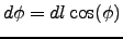
Figure (1.1) presents the
bottom topography obtained with make_grid.m for the
Southern Benguela example. Note that at this low
resolution (1/3), the topography has been strongly
smoothed.
Figure 1.1:
Result of make_grid.m for the Benguela example
 |
The next step is to create the file containing the different surface
fluxes. The part of the file romstools_param.m that you should edit is :
%
%%%%%%%%%%%%%%%%%%%%%%%%%%%
% 3-Surface forcing parameters
% used by make_forcing.m and by make_bulk.m
%
%%%%%%%%%%%%%%%%%%%%%%%%%%%
% COADS directory (for climatology runs)
%
coads_dir=[ROMSTOOLS_dir,'COADS05/'];
%
% COADS time (for climatology runs)
%
coads_time=(15:30:345); % days: middle of each month
coads_cycle=360; % repetition of a typical year of 360 days
%
%%%%%%%%%%%%%%%%%%%%%%%%%%%
%
% 3.1 Surface forcing parameters
% used by pathfinder_sst.m
%
%%%%%%%%%%%%%%%%%%%%%%%%%%%
%
pathfinder_sst_name=[ROMSTOOLS_dir,...
'SST_pathfinder/climato_pathfinder.nc'];
Variables description:
- coads_dir=[ROMSTOOLS_dir,'COADS05/'] : Directory where the global atlas of surface marine
data at 1/2 resolution (Da Silva et al., 1994) is located.
- coads_time=(15:30:345) : Time in days for the monthly climatology. It corresponds to the
middle of each month. ROMS uses this time to interpolate linearly the forcing variables in time.
- coads_cycle=360 : Duration on which the forcing variables are cycled. Here, for the sake
of simplicity, we are running the model on a repeating climatological year of 360 days.
- pathfinder_sst_name=[ROMSTOOLS_dir,SST_pathfinder/climato_pathfinder.nc'] :
Directory of the monthly climatology of sea surface temperature from Pathfinder satellite
observations (Casey and Cornillon, 1999). This can be used has an alternative of Da Silva et al. (1994) SST.
Save romstools_param.m and run make_forcing in the Matlab session :
make_forcing
You should obtain :
---------------------------------------------
Benguela Test Model
Read in the grid...
Create the forcing file...
Getting taux for time index 1
Getting tauy for time index 1
...
Make a few plots...
---------------------------------------------
This program can take a relatively long time to process all the forcing variables.
Figure (1.2) presents the wind stress vectors and wind stress norm
obtained from the global atlas of surface marine
data at 1/2 resolution (Da Silva et al., 1994) at 4 different periods of the year.
Da Silva et al. (1994) sea surface temperature (SST) is used for the restoring term (dQdSST)
in the heat flux calculation. To improve the model solution it is possible to
use a SST climatology at a finer resolution (9.28 km) (Casey and Cornillon, 1999). To do
so, you can run pathfinder_sst.m in the Matlab session :
pathfinder_sst
You should obtain :
---------------------------------------------
... Month index: 1
... Month index: 2
...
---------------------------------------------
For the surface forcing, instead of directly prescribing the fluxes, it is possible
to use a bulk formula to generate the surface fluxes from atmospheric variables
during the model run. In this case, ROMS needs to be recompiled with the BULK_FLUX
cpp key defined. To generate the bulk forcing file, you need to run make_bulk
in the Matlab session :
make_bulk
You should obtain :
---------------------------------------------
Benguela Test Model
Read in the grid...
Create the bulk forcing file...
Getting sat for time index 1
Getting sat for time index 2
...
Make a few plots...
---------------------------------------------
Figure 1.2:
Wind stress[N.m ] obtained using make_forcing.m for the Benguela example.
 |
The last preprocessing step consists in generating the files containing
the necessary informations for the ROMS initial and lateral open boundaries
conditions.
This script generates two files : the climatology file (XXX_clm.nc) which gives
the lateral boundary conditions, and the initial conditions file (XXX_ini.nc).
The part which should be edited by the user in the file romstools_param.m is. Note that you can
you can add the variables for the NPZD or PISCES biogeochemical models. For that,
define makebio or makepisces flags in the romstools_param.m.
The part which should be edited by the user in the file romstools_param.m is:
%%%%%%%%%%%%%%%%%%%%%%%%%%%%%%%
%
% 4-Open boundaries and initial conditions parameters
% used by make_clim.m, make_biol.m, make_bry.m
%
%%%%%%%%%%%%%%%%%%%%%%%%%%%%%%%
% Open boundaries switches (! should be consistent with cppdefs.h !)
%
obc = [1 1 1 1]; % open boundaries (1=open , [S E N W])
%
% Level of reference for geostrophy calculation
%
zref = -1000;
%
% Switches for selecting what to process in make_clim (1=ON)
% (and also in make_OGCM.m and make_OGCM_frcst.m)
makeini=1; %1: process initial data
makeclim=1; %1: process lateral boundary data
makebry=0; %1: process boundary data
makebio=0; %1: process initial and boundary data for idealized NPZD type bio model
makepisces=0; %1: process initial and boundary data for PISCES biogeochemical model
%
makeoa=1; %1: process oa data (intermediate file)
makeZbry=0; %1: process data in Z coordinate
%
insitu2pot=1; %1: convert in-situ temperature into potential temperature
%
% Day of initialization for climatology experiments (=0 : 1st January 0h)
%
tini=0;
%
% World Ocean Atlas directory (WOA2001 or WOA2005)
%
woa_dir=[ROMSTOOLS_dir,'WOA2005/'];
%
% Surface chlorophyll seasonal climatology (WOA2001 or SeaWifs)
%
chla_dir=[ROMSTOOLS_dir,'SeaWifs/'];
%
% Set times and cycles for the boundary conditions:
% monthly climatology
%
woa_time=(15:30:345); % days: middle of each month
woa_cycle=360; % repetition of a typical year of 360 days
%
Variables description:
- obc=[1 1 1 1] : Switches to open (1=open) or close (0=wall) the lateral
boundaries [South East North West]. This is used for the application of mass
enforcement. Be aware, this should be compatible with the open boundary
CPP-switches in the file /Roms_tools/Run/cppdefs.h.
- zref=-1000 : Depth [meters] of the level of no motion for the geostrophic
velocities calculation.
- makeini=1 : Switch to define if the initial file (roms_ini.nc) is generated.
Should be 1.
- makeclim=1 : Switch to define if the climatology
(lateral boundary conditions) file (roms_clm.nc) is generated. Should be 1.
- makeoa=1 : Switch to define if the OA (objective analysis; roms_oa.nc)
file is generated. This should be 1. The OA files are intermediate files
where hydrographic data are stored on a ROMS horizontal grid but on
a z vertical grid. The transformation into S-coordinate is done later.
This file is not used by ROMS.
- makebry=1 : Switch to define if the boundary file (roms_bry.nc) is generated.
Used only with make_bry.
- makeZbry=1 : Switch to define if the boundary intermediate file on a z coordinate
(roms_bry_Z.nc) is generated. Used only with make_bry.
- makebio=1; Switch to process initial and boundary data for idealized NPZD type bio model
- makepisces=1 : Switch to process initial and boundary data for PISCES biogeochemical model
- insitu2pot=1 : Switch defined if it is in-situ temperature that is provided.
In this case, in-situ temperature is converted into potential temperature.
- tini=0 : Day of initialization in climatology experiments (15 = January 15).
- woa_dir=[ROMSTOOLS_dir,'WOA2005/'] : Directory where the World Ocean
Atlas 2005 climatology (Conkright et al., 2002) is located. The World Ocean
Atlas 2001 climatology can also be used.
- chla_dir=[ROMSTOOLS_dir,'SeaWifs/'] : Directory of the surface
chlorophyll seasonal climatology.
- woa_time=(15:30:345) : Time in days for the WOA monthly climatology.
It corresponds to the middle of each month. ROMS uses this variable to
interpolate linearly the climatology variables in time.
- woa_cycle=360 : Duration on which the climatology variables are cycled.
Here, for the sake of simplicity, we are running the model on a repeating climatological
year of 360 days.
Save romstools_param.m and run make_clim in the Matlab session :
make_clim
You should obtain :
---------------------------------------------
Making the clim: ../Run/ROMS_FILES/roms_clm.nc
Title: Benguela Test Model
Read in the grid...
Create the climatology file...
Creating the file : ../Run/ROMS_FILES/roms_clm.nc
...
Make a few plots...
---------------------------------------------
This program can also take quite a long time to run.
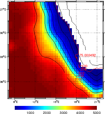
Figure (1.3) presents 4 different sections
of temperature for the initial condition file for the
Benguela example. The sections are in the X-direction (East-West),
the first section is for the Southern part of the domain and the last one
is for the Northern part of the domain.
Figure 1.3:
Result of make_clim.m for the Benguela example
 |
An alternative of using a climatology file is to create a boundary
file. In this case, only boundary values are stored. The cpp key
FRC_BRY should be defined and ROMS recompiled. Run make_bry in
the Matlab session :
make_bry
You should obtain :
---------------------------------------------
Making the file: ../Run/ROMS_FILES/roms_bry.nc
Title: Benguela Test Model
Read in the grid...
...
---------------------------------------------
Once all the netcdf data files are ready (i.e. XXX_grd.nc,
XXX_frc.nc, XXX_ini.nc, and XXX_clm.nc), we can prepare ROMS for
compilation. All is done in the /Roms_tools/Run/ directory.
Edit the file /Roms_tools/Run/param.h.
The line which needs to be changed is:
# elif defined BENGUELA_LR
parameter (LLm0=41, MMm0=42, N=32) !  Southern Benguela Test Case
# else
These are the values of the model grid size: LLm0 points in the X direction, MMm0
points in the Y direction and N vertical levels. LLm0 and MMm0 are given by running
make_grid.m, and N is defined in romstools_param.m. The param.h parameters are
described in detail in section 2.4
The second file to edit is /Roms_tools/Run/cppdefs.h. This file defines the
CPP keys that are used by the the C-preprocessor when compiling ROMS. The
C-preprocessor selects the different parts of the Fortran code which needs to be
compiled depending on the defined CPP options. These options are separated in two
parts (the basic option keys and the advanced options keys) in cppdefs.h. All the
keys and their organization are described in section 2.5.
ROMS can be compiled by running the UNIX tcsh script /Roms_tools/Run/jobcomp.
Jobcomp should be able to recognize your system. It has been tested on Linux, IBM,
Sun and Compaq systems. On Linux PCs, the default compiler is the GNU g77, but it is
possible to uncomment specific lines in jobcomp to use g95 or ifort. The latter is
mandatory when using AGRIF and/or OPEN_MP. When changing the compiler you should
provide a corresponding NetCDF library. Once the compilation is done, you should
obtain a new executable (roms) in the /Roms_tools/Run directory. ROMS should
be recompiled each time param.h or cppdefs.h are changed. If you compile using MPI
parallelization, the jobcomp scrip detect it and set the compiler to OpenMPI, so you
need to have it installed (http://www.open-mpi.org)
Edit the input parameter file: /Roms_tools/Run/roms.in. The vertical grid
parameters (THETA_S, THETA_B, HC) should be identical to the ones in
romstools_param.m. Otherwise, the other default values should not be changed. The
definition of all the input variables is given at the start of each ROMS simulation.
To run the model, type in directory /Roms_tools/Run/ : ./roms roms.in.
If you use paralelle computation, some more specific command are needed :
in the case of OpenMP parallelization, set the environment variable OMP_NUM_THREADS
to number_of_cpu_used (for example export OMP_NUM_THREADS=4 for 4 cpu
parallel run) then ./roms roms.in. In the case of MPI parallelization, use the
following command : mpirun -np number_of_processus_used ./roms roms.in.
The description of the namelist roms.in is descibed in details in section
2.6.
On the screen, you should check the Cu_max parameter: if it is greater than 1 you
are violating the CFL criterion. In this case, you should reduce the time step.
Example of model run:
: ./roms roms.in
You should obtain :
---------------------------------------------
Southern Benguela
480 ntimes Total number of timesteps for 3D equations.
5400.00 dt Timestep [sec] for 3D equations
60 ndtfast Number of 2D timesteps within each 3D step.
1 ninfo Number of timesteps between runtime diagnostics.
6.000E+00 theta_s S-coordinate surface control parameter.
0.000E+00 theta_b S-coordinate bottom control parameter.
1.000E+01 Tcline S-coordinate surface/bottom layer width used in
vertical coordinate stretching, meters.
Grid File: ROMS_FILES/roms_grd.nc
Forcing Data File: ROMS_FILES/roms_frc.nc
Bulk Data File: ROMS_FILES/roms_blk.nc
Climatology File: ROMS_FILES/roms_clm.nc
Initial State File: ROMS_FILES/roms_ini.nc Record: 1
Restart File: ROMS_FILES/roms_rst.nc nrst = 480 rec/file: -1
History File: ROMS_FILES/roms_his.nc Create new: T nwrt = 480 rec/file = 0
1 ntsavg Starting timestep for the accumulation of output
time-averaged data.
48 navg Number of timesteps between writing of time-averaged
data into averages file.
Averages File: ROMS_FILES/roms_avg.nc rec/file = 0
Fields to be saved in history file: (T/F)
T write zeta free-surface.
F write UBAR 2D U-momentum component.
F write VBAR 2D V-momentum component.
F write U 3D U-momentum component.
F write V 3D V-momentum component.
F write T(1) Tracer of index 1.
F write T(2) Tracer of index 2.
F write RHO Density anomaly.
F write Omega Omega vertical velocity.
F write W True vertical velocity.
F write Akv Vertical viscosity.
F write Akt Vertical diffusivity for temperature.
F write Aks Vertical diffusivity for salinity.
F write Hbl Depth of KPP-model boundary layer.
F write Bostr Bottom Stress.
Fields to be saved in averages file: (T/F)
T write zeta free-surface.
T write UBAR 2D U-momentum component.
T write VBAR 2D V-momentum component.
T write U 3D U-momentum component.
T write V 3D V-momentum component.
T write T(1) Tracer of index 1.
T write T(2) Tracer of index 2.
F write RHO Density anomaly
T write Omega Omega vertical velocity.
T write W True vertical velocity.
F write Akv Vertical viscosity
T write Akt Vertical diffusivity for temperature.
F write Aks Vertical diffusivity for salinity.
T write Hbl Depth of KPP-model boundary layer
T write Bostr Bottom Stress.
1025.0000 rho0 Boussinesq approximation mean density, kg/m3.
0.000E+00 visc2 Horizontal Laplacian mixing coefficient [m2/s]
for momentum.
0.000E+00 tnu2(1) Horizontal Laplacian mixing coefficient (m2/s)
for tracer 1.
0.000E+00 tnu2(2) Horizontal Laplacian mixing coefficient (m2/s)
for tracer 2.
0.000E+00 rdrg Linear bottom drag coefficient (m/si).
0.000E+00 rdrg2 Quadratic bottom drag coefficient.
1.000E-02 Zob Bottom roughness for logarithmic law (m).
1.000E-04 Cdb_min Minimum bottom drag coefficient.
1.000E-01 Cdb_max Maximum bottom drag coefficient.
1.00 gamma2 Slipperiness parameter: free-slip +1, or no-slip -1.
1.00E+05 x_sponge Thickness of sponge and/or nudging layer (m)
800.00 v_sponge Viscosity in sponge layer (m2/s)
1.157E-05 tauT_in Nudging coefficients [sec-1]
3.215E-08 tauT_out Nudging coefficients [sec-1]
1.157E-06 tauM_in Nudging coefficients [sec-1]
3.215E-08 tauM_out Nudging coefficients [sec-1]
Activated C-preprocessing Options:
REGIONAL
BENGUELA_LR
OBC_EAST
OBC_WEST
OBC_NORTH
OBC_SOUTH
SOLVE3D
UV_COR
UV_ADV
CURVGRID
SPHERICAL
MASKING
UV_VIS2
MIX_GP_UV
MIX_GP_TS
TS_DIF2
LMD_MIXING
LMD_SKPP
LMD_BKPP
LMD_RIMIX
LMD_CONVEC
SALINITY
NONLIN_EOS
SPLIT_EOS
QCORRECTION
SFLX_CORR
DIURNAL_SRFLUX
SPONGE
CLIMATOLOGY
ZCLIMATOLOGY
M2CLIMATOLOGY
M3CLIMATOLOGY
TCLIMATOLOGY
ZNUDGING
M2NUDGING
M3NUDGING
TNUDGING
ANA_BSFLUX
ANA_BTFLUX
OBC_M2CHARACT
OBC_M3ORLANSKI
OBC_TORLANSKI
AVERAGES
AVERAGES_K
VAR_RHO_2D
M2FILTER_POWER
CLIMAT_UV_MIXH
VADV_SPLINES_UV
HADV_UPSTREAM_TS
CLIMAT_TS_MIXH
VADV_AKIMA_TS
 Non user defined cpp keys (in set_global_definitions.h)
DBLEPREC
Linux
QUAD
QuadZero
GLOBAL_2D_ARRAY
GLOBAL_1D_ARRAYXI
GLOBAL_1D_ARRAYETA
...
...
AGRIF_UPDATE_DECAL
AGRIF_SPONGE
Linux 2.6.9-42.0.3.ELsmp x86_64
NUMBER OF THREADS: 1 BLOCKING: 1 x 1.
Spherical grid detected.
hmin hmax grdmin grdmax Cu_min Cu_max
75.000000 4803.032721 .301836927E+05 .331215714E+05 0.12176008 0.91533005
volume=9.523986093261087500000E+14 open_cross=6.104836888312444686890E+09
Vertical S-coordinate System:
level S-coord Cs-curve at_hmin over_slope at_hmax
32 0.0000000 0.0000000 0.000 0.000 0.000
31 -0.0312500 -0.0009350 -0.373 -2.584 -4.794
30 -0.0625000 -0.0019030 -0.749 -5.247 -9.746
29 -0.0937500 -0.0029380 -1.128 -8.074 -15.019
28 -0.1250000 -0.0040767 -1.515 -11.152 -20.790
27 -0.1562500 -0.0053591 -1.911 -14.580 -27.249
26 -0.1875000 -0.0068304 -2.319 -18.466 -34.613
25 -0.2187500 -0.0085426 -2.743 -22.938 -43.132
24 -0.2500000 -0.0105560 -3.186 -28.141 -53.095
23 -0.2812500 -0.0129416 -3.654 -34.248 -64.842
22 -0.3125000 -0.0157835 -4.151 -41.463 -78.776
21 -0.3437500 -0.0191819 -4.684 -50.031 -95.377
20 -0.3750000 -0.0232566 -5.262 -60.241 -115.220
19 -0.4062500 -0.0281514 -5.892 -72.443 -138.993
18 -0.4375000 -0.0340388 -6.588 -87.056 -167.524
17 -0.4687500 -0.0411263 -7.361 -104.584 -201.807
16 -0.5000000 -0.0496640 -8.228 -125.635 -243.041
15 -0.5312500 -0.0599527 -9.209 -150.939 -292.668
14 -0.5625000 -0.0723554 -10.328 -181.377 -352.427
13 -0.5937500 -0.0873092 -11.613 -218.013 -424.414
12 -0.6250000 -0.1053416 -13.097 -262.126 -511.156
11 -0.6562500 -0.1270882 -14.823 -315.262 -615.700
10 -0.6875000 -0.1533158 -16.841 -379.282 -741.723
9 -0.7187500 -0.1849493 -19.209 -456.432 -893.656
8 -0.7500000 -0.2231040 -22.002 -549.423 -1076.845
7 -0.7812500 -0.2691252 -25.306 -661.522 -1297.738
6 -0.8125000 -0.3246355 -29.226 -796.670 -1564.114
5 -0.8437500 -0.3915923 -33.891 -959.622 -1885.352
4 -0.8750000 -0.4723564 -39.453 -1156.112 -2272.770
3 -0.9062500 -0.5697755 -46.098 -1393.057 -2740.015
2 -0.9375000 -0.6872846 -54.048 -1678.800 -3303.552
1 -0.9687500 -0.8290268 -63.574 -2023.407 -3983.240
0 -1.0000000 -1.0000000 -75.000 -2439.016 -4803.033
Time splitting: ndtfast = 60 nfast = 89
Maximum grid stiffness ratios: rx0 =0.2353349875 rx1 = 2.5672736953
GET_INITIAL - Processing data for time = 0.000 record = 1
GET_TCLIMA - Read climatology of tracer 1 for time = 345.0
GET_TCLIMA - Read climatology of tracer 1 for time = 15.00
GET_TCLIMA - Read climatology of tracer 2 for time = 345.0
GET_TCLIMA - Read climatology of tracer 2 for time = 15.00
GET_UCLIMA - Read momentum climatology for time = 345.0
GET_UCLIMA - Read momentum climatology for time = 15.00
GET_SSH - Read SSH climatology for time = 345.0
GET_SSH - Read SSH climatology for time = 15.00
GET_SMFLUX - Read surface momentum stresses for time = 345.0
GET_SMFLUX - Read surface momentum stresses for time = 15.00
GET_BULK - Read fields for bulk formula for time = 345.0
GET_BULK - Read fields for bulk formula for time = 15.00
DEF_HIS/AVG - Created new netCDF file 'ROMS_FILES/roms_his.nc'.
WRT_GRID - wrote grid data into file 'ROMS_FILES/roms_his.nc'.
WRT_HIS - wrote history fields into time record = 1 / 1
MAIN: started time-steping.
STEP time[DAYS] KINETIC_ENRG POTEN_ENRG TOTAL_ENRG NET_VOLUME trd
0 0.00000 0.000000000E+00 2.1475858E+01 2.1475858E+01 9.5239861E+14 0
1 0.06250 1.306369099E-04 2.1476230E+01 2.1476361E+01 9.5239208E+14 0
...
---------------------------------------------
In many studies, there is a need for long simulations: to reach the spin-up of
the solution and/or to obtain statistical equilibriums.
For regional models, 10 years appears to be a reasonable model simulation length.
In this case, to prevent the generation of large output files, the strategy
is to relaunch the model every simulated month.
This is done by the UNIX csh script: run_roms.csh .
Warning! the ROMS input file use for long simulations is roms_inter.in.
It should be edited accordingly.
- It gets the grid, the forcing, the initial and the boundary files.
- It runs the model for 1 month.
- It stores the output files in a specific form: roms_avg_Y4M3.nc (for the ROMS
averaged output of March of year 4).
- It replaces the initial file by the restart file (roms_rst.nc) which as
been generated at the end of the month.
- It relaunch the model for next month.
Part to edit in run_roms.csh:
set MODEL=roms
set SCRATCHDIR=`pwd`/SCRATCH
set INPUTDIR=`pwd`
set MSSDIR=`pwd`/ROMS_FILES
set MSSOUT=`pwd`/ROMS_FILES
set CODFILE=roms
set AGRIF_FILE=AGRIF_FixedGrids.in
#
# Model time step [seconds]
#
set DT=5400
#
# Number of days per month
#
set NDAYS = 30
#
# number total of grid levels
#
set NLEVEL=1
#
# Time Schedule - TIME_SCHED=0 - yearly files
# TIME_SCHED=1 - monthly files
#
set TIME_SCHED=1
#
set NY_START=1
set NY_END=10
set NM_START=1
set NM_END=12
Variables definitions:
- MODEL=roms : Name used for the input files. For example roms_grd.nc.
- SCRATCHDIR=`pwd`/SCRATCH : Scratch directory where the model is run
- INPUTDIR=`pwd` : Input directory where the roms_inter.in input file
is.
- MSSDIR=`pwd`/ROMS_FILES : Directory where the roms input NetCDF files
(roms_grd.nc, roms_frc.nc, ...) are stored.
- MSSOUT=`pwd`/ROMS_FILES : Directory where the roms output NetCDF files
(roms_his.nc, roms_avg.nc, ...) are stored.
- CODFILE=roms : ROMS executable.
- AGRIF_FILE=AGRIF_FixedGrids.in : AGRIF input file which defines the
position of child grids when using embedding.
- DT=5400 : Model time step in seconds.
- NDAYS = 30 : Number of days in 1 month.
- NLEVEL=1 : Total number of model grids (no AGRIF: NLEVEL=1).
- NY_START=1 : Starting year.
- NY_END=10 : Ending Year.
- NM_START=1 : Starting month.
- NM_END=12 : Ending month.
To run a ROMS long simulation in batch mode on a Linux workstation:
: nohup ./run_roms.csh exp1.out &
To check the execution of your model, type in the directory
/Roms_Tools/Run :
: more exp1.out
Once the model has run, or during the simulation, it is possible
to visualize the model outputs using a Matlab graphic user interface :
roms_gui. Launch roms_gui in the Matlab session
(in the /Roms_tools/Run/ directory):
roms_gui
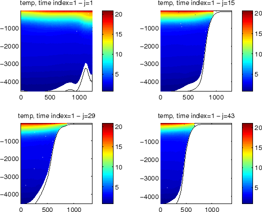
A window pops up, asking for a ROMS history NetCDF file (Figure 1.4).
You should select roms_his.nc (history file) or roms_avg.nc (average file) and
click "open".
Figure 1.4:
Entrance window of roms_gui
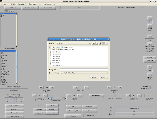 |
Figure 1.5:
roms_gui
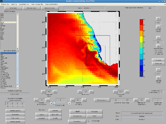 |
The main window appears, variables can be selected to obtain an image such as
Figure (1.5). On the left side, the upper box gives the available
ROMS variable names and the lower box presents the variables derived from the
ROMS model outputs :
- Ke : Horizontal slice of kinetic energy:
 .
.
- Rho : Horizontal slice of density using the non-linear equation of state
for seawater of Jackett and McDougall (1995).
- Pot_Rho : Horizontal slice of the potential density.
- Bvf : Horizontal slice of the Brunt-Väisäla frequency:

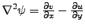
- Vort : Horizontal slice of vorticity:
 .
.
- Pot_vort : Horizontal slice of the vertical component of Ertel's potential vorticity:
![$\frac{\partial \lambda}{\partial z} \left [ f +
\left (\frac{\partial v}{\partial x}-\frac{\partial u}{\partial y}\right ) \right ]$](img33.png) .
In our case,
.
In our case,  .
.
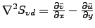
- Psi : Horizontal slice of stream function:
 .
This routine might be costly since it inverses the Laplacian of the vorticity
(using a successive over relaxation solver).
.
This routine might be costly since it inverses the Laplacian of the vorticity
(using a successive over relaxation solver).
- Speed : Horizontal slice of the ocean currents velocity :
 .
.
- Transport : Horizontal slice of the transport stream function :
 .
.
- Okubo : Horizontal slice of the Okubo-Weiss parameter :
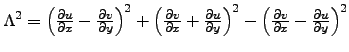 .
.
- Chla : Compute a chlorophyll-a from Large and Small phytoplankton concentrations.
- z_SST_1C : Depth of 1C below SST.
- z_rho_1.25 : Depth of 1.25 kg.m
 below surface density.
- z_max_bvf : Depth of the maximum of the Brunt-Väisäla frequency.
- z_max_dtdz : Depth of the maximum vertical temperature gradient.
- z_20C : Depth of the 20C isotherm.
- z_15C : Depth of the 15C isotherm.
- z_sig27 : Depth of the 1027 kg.m density layer.
- r_factor :
It is possible to add arrows for the horizontal currents by increasing the "Current vectors
spatial step". It is also possible to obtain vertical sections, time series, vertical profiles
and Hovmüller diagrams by clicking on the corresponding targets in roms_gui.
To analyze the long simulations,
a few scripts have been added in the directory:
/Roms_tools/Diagnostic_tools:
- roms_diags.m : Get volume and surface averaged quantities from a ROMS simulation.
- plot_diags.m : Plot the averaged quantities computed by roms_diags.m.
- get_Mmean.m : Get the monthly mean climatology.
- get_Smean.m : Get the seasonal and annual mean climatology from the outputs of
get_Mmean.m.
- get_Meddy.m : Get the monthly variance climatology (if the variable nonseannal = 1,
the non-seasonal variance is computed; i.e., the seasonal variation are
filtered). It needs that get_Mmean.m and get_Smean.m are run before.
- get_Seddy.m : Get the seasonal and annual RMS from the results of
get_Meddy.m.
- roms_anim.m : Create an animation from the monthly history or average files.
Run these scripts in a Matlab session.
The obtained mean or eddy files can be visualized with roms_gui.
If you need to create and play ".fli" animations, you should install ppm2fli
and xanim on your system. If you have a Linux PC, you can follow these steps:
- log in as root
- go to the directory where the file is saved.
- type : rpm -Uvh ppm2fli-2.1-1.i386.rpm
- type : rpm -Uvh xanim-2.80.1-12.i386.rpm
- log out
If you are not using a Linux PC, you should ask your
system administrator to install these programs.
Using the method described by Flather (1976), ROMS is able to propagate the
different tidal constituents from its lateral boundaries. To do so, define
the cpp keys TIDES, SSH_TIDES and UV_TIDES and recompile the model
using jobcomp. To work correctly, the model should use the Flather (1976)
open boundary radiation scheme (cpp key OBC_M2FLATHER defined).
The tidal components are added to the forcing file (XXX_frc.nc)
by the Matlab program make_tides.m.
Edit the file : /Roms_tools/Run/romstools_param.m.
The part of the file that you should change is :
%%%%%%%%%%%%%%%%%%%%%
%
% 5-Parameters for tidal forcing
%
%%%%%%%%%%%%%%%%%%%%%
%
% TPXO file name (TPXO6 or TPXO7)
%
tidename=[ROMSTOOLS_dir,'TPXO6/TPXO6.nc'];
%
% Number of tides component to process
%
Ntides=10;
%
% Chose order from the rank in the TPXO file :
% "M2 S2 N2 K2 K1 O1 P1 Q1 Mf Mm"
% " 1 2 3 4 5 6 7 8 9 10"
%
tidalrank=[1 2 3 4 5 6 7 8 9 10];
%
% Compare with tidegauge observations
%
lon0=18.37;
lat0=-33.91; % Cape Town location
Z0=1; % Mean depth of the tidegauge in Cape Town
Variables definitions :
- tidename=[ROMSTOOLS_dir,'TPXO6/TPXO6.nc'] : Location of the netcdf tidal dataset.
This file is derived from the Oregon State University global model of ocean tides TPXO.6
(Egbert and Erofeeva, 2002). Data sources can be found at
http://www.oce.orst.edu/po/research/tide/global.html.
It is also possible to use TPXO7.
- Ntides=10 : Number of tidal components to process. Warning!
This value should be identical to the value of the parameter Ntides in param.h:
"parameter (Ntides=10)".
- tidalrank=[1 2 3 4 5 6 7 8 9 10] : Order to select the different tidal components.
- lon0=18.37;lat0=-33.91;Z0=1 : Location of a tidal gauge to compare the interpolated values
with observations.
An important aspect is the definition of time and especially the choice of a
time origin. This is defined in /Roms_tools/Run/romstools_param.m:
%%%%%%%%%%%%%%%%%%%%%%%%%%
%
% 6-Temporal parameters (used for make_tides, make_NCEP, make_OGCM)
%
%%%%%%%%%%%%%%%%%%%%%%%%%%%%%%%%%%%%%%%%
%
Yorig = 1900; % reference time for vector time
% in roms initial and forcing files
%
Ymin = 2000; % first forcing year
Ymax = 2000; % last forcing year
Mmin = 1; % first forcing month
Mmax = 3; % last forcing month
%
Dmin = 1; % Day of initialization
Hmin = 0; % Hour of initialization
Min_min = 0; % Minute of initialization
Smin = 0; % Second of initialization
%
SPIN_Long = 0; % SPIN-UP duration in Years
%
The origin of time (Yorig: 1 january of year Yorig) should be kept the same
for all the preprocessing and postprocessing steps.
Save romstools_param.m and run make_tides in the Matlab session:
make_tides
You should obtain :
---------------------------------------------
Start date for nodal correction : 1-Jan-2000
Reading ROMS grid parameters ...
Tidal components : M2 S2 N2 K2 K1 O1 P1 Q1 Mf Mm
Processing tide : 1 of 10
...
---------------------------------------------
ROMSTOOLS can help for the design of ROMS biogeochemical
experiments. For the initial conditions and lateral boundary
conditions, WOA provides a seasonal climatology for nitrateD
concentration and WOA or SeaWifs can be used to obtain a
seasonal climatology of surface chlorophyll concentration.
Phytoplankton is estimated by a constant chlorophyll/phytoplankton
ratio derived from previous simulations. Zooplankton is estimated
in a similar way. The part which should be edited by the user in
romstools_param.m is:
%%%%%%%%%%%%%%%%%%%%%%%%%%%%%%%
%
% Open boundaries and initial conditions parameters
% used by make_clim.m, make_biol.m, make_bry.m
%%%%%%%%%%%%%%%%%%%%%%%%%%%%%%%
.....
makebio=1; %1: process initial and boundary data for idealized NPZD type bio model
.....
%
% World Ocean Atlas directory (WOA2001 or WOA2005)
%
woa_dir=[DATADIR,'WOA2005/'];
%
% Pisces biogeochemical seasonal climatology (WOA2001 or WOA2005)
%
woapisces_dir=[DATADIR,'WOAPISCES/'];
%
% Surface chlorophyll seasonal climatology (WOA2001 or SeaWifs)
%
chla_dir=[DATADIR,'SeaWifs/'];
%
....
Variables description :
- woa_dir=[ROMSTOOLS_dir,'WOA2005/'] : Directory where the World Ocean
Atlas 2005 climatology (Conkright et al., 2002) is located. The World Ocean
Atlas 2001 climatology can also be used.
- chla_dir=[ROMSTOOLS_dir,'SeaWifs/'] : Directory of the surface
chlorophyll seasonal climatology.
Run make_biol (or if the flag makebio=1,
make_clim.m will process make_biol.m )
in the Matlab session :
make_biol
You should obtain :
----------------------------------------
Add_no3: creating variables and attributes for the OA file
Add_no3: creating variables and attributes for the Climatology file
Ext tracers: Roa = 0 km - default value = NaN
Ext tracers: horizontal interpolation of the annual data
Ext tracers: horizontal interpolation of the seasonal data
time index: 1 of total: 4
time index: 2 of total: 4
time index: 3 of total: 4
time index: 4 of total: 4
Vertical interpolations
NO3...
Time index: 1 of total: 4
Time index: 2 of total: 4
Time index: 3 of total: 4
Time index: 4 of total: 4
CHla...
Add_chla: creating variable and attribute
...
Make a few plots...
----------------------------------------
The cpp keys related to these biology models are :
- BIO_NChlPZD : Select a 5 components (Nitrate, Chlorophyll, Phytoplankton,
Zooplankton, Detritus) biogeochemical model.
- BIO_N2ChlPZD2 : Select a 7 components (Nitrate, Ammonium, Chlorophyll,
Phytoplankton, Zooplankton, Small Detritus, Large Detritus) biogeochemical model.
- BIO_N2P2Z2D2 : Select a 8 components (Nitrate, Ammonium, Small
Phytoplankton, Large Phytoplankton, Small Zooplankton, Large Zooplankton,
Small Detritus, Large Detritus) biogeochemical model.
- DIAGNOSTICS_BIO : Define if writing out fluxes between the biological
components.
This latter is a more complex biogeochemical model, firstly coupled to OPA and now a
beta version of the model can be coupled with ROMS_AGRIF. It is nicely
described in (Aumont , 2005) provide in the documentation section of
ROMS_TOOLS.
This part of ROMS_TOOLS use the World Ocean Atlas, called WOAPISCES. It provides the global data of Iron (Fe), Silicate (SiO3), Oxygen (O2), Phosphate (PO4), DIC (dissolved organic
carbon), DOC (dissolved inorganic carbon) and Alkanility. The routines used to process these fields are : make_ini_pisces, make_clim_pisces, make_bry_pisces, make_bio_forcing.m as for the climatological experiments1.1.
The part which should be edited by the user in romstools_param.m is:
%%%%%%%%%%%%%%%%%%%%%%%%%%%%%%%
%
% Open boundaries and initial conditions parameters
% used by make_clim.m, make_biol.m, make_bry.m
%%%%%%%%%%%%%%%%%%%%%%%%%%%%%%%
.....
makepisces %1: process initial and boundary data for PISCES biogeochemical model
.....
%
% Pisces biogeochemical seasonal climatology (WOA2001 or WOA2005)
%
woapisces_dir=[DATADIR,'WOAPISCES/'];
%
....
Variables description :
- woapisces=[DATADIR,'WOAPISCES/'] : Directory where the World Ocean
Atlas 2005 climatology is located. It contains the variable needed by PISCES biogeochemical model.
To add boundary conditions of PISCES in the roms_clm.nc computed before, in a matlab session, run make_clim_pisces.
make_clim_pisces
You should obtain :
Add_no3: creating variables and attributes for the OA file
write no3time
Add_po4: creating variables and attributes for the OA file
Add_sio3: creating variables and attributes for the OA file
Add_o2: creating variables and attributes for the OA file
Add_dic: creating variables and attributes for the OA file
Add_talk: creating variables and attributes for the OA file
Add_doc: creating variables and attributes for the OA file
Add_fer: creating variables and attributes for the OA file
Ext tracers: Roa = 0 km - default value = NaN
Ext tracers: horizontal interpolation of the seasonal data
time index: 1 of total: 12
time index: 2 of total: 12
time index: 3 of total: 12
time index: 4 of total: 12
time index: 5 of total: 12
time index: 6 of total: 12
time index: 7 of total: 12
time index: 8 of total: 12
time index: 9 of total: 12
time index: 10 of total: 12
time index: 11 of total: 12
time index: 12 of total: 12
Similarly, to add initial condition for PISCES variables to roms_ini.nc file, in a matlab session, run make_ini_pisces.m
make_ini_pisces
Figure 1.6:
Result of make_clim_pisces for the Benguela example : NO3 forcing
fields [mMol N m-3].
[Surface map]
![\includegraphics[width=0.5\textwidth]{Figures/NO3_surf_t1.eps}](img41.png) [vertical sections along open boundaries]
[vertical sections along open boundaries]
![\includegraphics[width=0.5\textwidth]{Figures/NO3_profil_t1.eps}](img42.png) |
Figure 1.7:
Result of make_clim_pisces for the Benguela example : PO4 forcing fields
[mMol P m-3].
[Surface map]
![\includegraphics[width=0.5\textwidth]{Figures/PO4_surf_t1.eps}](img43.png) [vertical sections along open boundaries]
[vertical sections along open boundaries]
![\includegraphics[width=0.5\textwidth]{Figures/PO4_profil_t1.eps}](img44.png) |
Finally, to compute the Iron dust deposition forcing file roms_frcbio.nc file, in a matlab session, run make_dust.m :
make_dust
Figure 1.8:
Result of make_clim_pisces for the Benguela example : Iron dust deposition
forcing fields [nmol Fe m-3].
|
If the makepisces =1 in romstools_param.m, make_clim.m will process directly make_clim_pisces.m, make_dust.m and eventually make_ini_pisces.m.
It is exactly the same procedure for the roms_bry.nc files.
The cpp keys related to this biogeochemical model are :
- PISCES : Select the PISCES biogeochemical model
- DIAGNOSTICS_BIO : Define if writing out fluxes between the biological
components.
ROMSTOOLS can help to realize inter-annual simulations. In this context,
we rely on Ocean Global Circulations Models (OGCM) for the lateral
boundary conditions and a global atmospheric reanalysis for the surface
forcing (NCEP). To limit the volume of data which needs to be transfered
over the Internet, we use Opendap to extract only the necessary subgrids.
The Matlab script make_NCEP.m is used to obtain the surface forcing data. It
downloads the necessary NCEP surface forcing data (Sea Surface Temperature, Wind
stress ...) over the Internet, and interpolates them on the model grid. Since
make_NCEP.m works with the bulk parameterization (i.e. the BULK_FLUX and BULK_EP
cpp keys should be defined in cppdefs.h), a surface forcing NetCDF file and a bulk
NetCDF file are generated for each month of your simulation in the directory
/Roms_tools/Run/ROMSFILES/ .
The part of the file romstools_param.m that you should change is:
%
%%%%%%%%%%%%%%%%%%%%%%%%%%%%%%%%%%
%
% 7 Parameters for Interannual forcing (SODA, ECCO, NCEP, ...)
%
%%%%%%%%%%%%%%%%%%%%%%%%%%%%%%%%%%
Download_data = 1; % Get data from the OPENDAP sites
level = 0; % AGRIF level; 0=parent grid
%
NCEP_version = 2; % NCEP version:
% 1: NCEP/NCAR Reanalysis, 1/1/1948 - present
% 2: NCEP-DOE Reanalysis, 1/1/1979 - present
%
% Path and option for using global datasets download from ftp
%
Get_My_Data = 0;
%
if NCEP_version == 1;
My_NCEP_dir = [DATADIR,'NCEP_REA1/'];
elseif NCEP_version == 2;
My_NCEP_dir = [DATADIR,'NCEP_REA2/'];
end
My_QSCAT_dir = [DATADIR,'QSCAT/'];
My_SODA_dir = [DATADIR,'SODA/'];
My_ECCO_dir = [DATADIR,'ECCO/'];
%======================================
%Options for make_NCEP and make_QSCAT_daily
%
NCEP_dir= [FORC_DATA_DIR,'NCEP_',ROMS_config,'/']; % NCEP data directory
makefrc = 1; % 1: Create forcing files
makeblk = 1; % 1: Create bulk files
QSCAT_blk = 1; % Correct NCEP frc/bulk file with the u,v,wspd fields from QSCAT daily
data. Download u, v, wspd in the QSCAT frc file
add_tides = 0; % 1: Add the tides (To be done...)
%Overlap parameters :
itolap_qscat=11; %11 days if 1d time reso. QSCAT (should be <28 )
itolap_ncep=40; %10 days if 6h time res. NCEP (should be <4* 28 =112
% ...
Variables description :
- FORC_DATA_DIR : Directory where the different files downloaded over
the Internet are stored.
- Download_data : Get data from the OPENDAP sites. Should be 1.
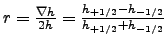
- level : AGRIF level. The parent grid = 0 and the child grid = 1.
- NCEP_dir= [FORC_DATA_DIR,'NCEP_',ROMS_config,'/'] : NCEP data directory.
This is where NCEP data downloaded over the Internet are stored.
- makefrc : Switch to define if the forcing file is generated. Should be 1.
- makeblk : Switch to define if the bulk file is generated. Should be 1.
- add_tides : Switch to define if the tidal forcing is added.
- NCEP_version : version of the NCEP reanalysis. 1: NCEP/NCAR Reanalysis, 1/1/1948 - present.
2: NCEP-DOE Reanalysis, 1/1/1979 - 12/31/2001.
- Get_My_Data = 1
- My_NCEP_dir = Path to local global NCEP datasets
- QSCAT_blk = Flag to use the QiuikSCAT wind in the NCEP bulk files
- itolap_qscat = Overlap parameters for the monthly roms forcing files using
QuikSCAT daily wind stress.
The overlap parameter is the number of "recovering"
time steps between 2 consecutives months
- itolap_ncep = Overlap parameters for the monthly roms forcing (and/or bulk files) using NCEP1 or
NCEP2 wind stress( and/or heat fluxes) monthly file
Save romstools_param.m and run make_NCEP in the Matlab session.
You should obtain:
make_NCEP
Read in the grid ROMS_FILES/roms_grd.nc

BEGIN DOWNLOAD STEP
Download NCEP data with OPENDAP or my FTP data
OPENDAP Procedure
Get NCEP data from 2000 to 2000
From http://nomad1.ncep.noaa.gov:9090/dods/reanalyses/reanalysis-2/
Minimum Longitude: 8
Maximum Longitude: 22
Minimum Latitude: -38
Maximum Latitude: -25.8968
Making output data directory
......./Run/DATA/NCEP_Benguela_LR/

VNAME IS landsfc
Get time units and time: Get_My_Data is OFF
Reading: http://nomad1.ncep.noaa.gov:9090/dods/reanalyses/reanalysis-2/6hr/flx/flx
Constraint: time
Server version: dods/3.2
...
make_NCEP
Read in the grid ROMS_FILES/roms_grd.nc

Download NCEP data with OPENDAP or my FTP data
Direct FTP Procedure
Use my own ncep data NCEP
Get NCEP data from  to
to
From path/NCEP_REA2/
Minimum Longitude: 
Maximum Longitude: 
Minimum Latitude: 
Maximum Latitude: 
Get_My_Data = 1
Read subgrid from file/data1/gcambon/NCEP_REA2/land.sfc.gauss.nc
Get the Land Mask tindex = 1
In case of Get_My_Data ON
Get the Land Mask by using extract_NCEP_Mask_Mydata
Execute extract_NCEP_Mask_Mydata
Get land for year 2000 - month 1
Create path/Run/DATA/NCEP_Benguela_LR/land_Y2000M1.nc
VNAME IS air
Processing year: 2000
1.8.2.1 QuikSCAT daily data from Ifremer OpenDap server
Similarly, The Matlab script make_QuickSCAT_daily.m is used to obtain the daily
surface stress forcing provided by the OpenDAP server at Ifremer, France:
http://www.ifremer.fr/dodsG/CERSAT/quikscat_daily.
A surface forcing NetCDF file NetCDF file is generated for each month of your
simulation in the directory /Roms_tools/Run/ROMSFILES/.
You shoud edit this part of the file romstools_param.m:
%%%%%%%%%%%%%%%%%%%%%%%%%%%%%%%%%%%%%%%
%
% 7 Parameters for Interannual forcing (SODA, ECCO, NCEP, ...)
%
%%%%%%%%%%%%%%%%%%%%%%%%%%%%%%%%%%%%%%%
%
% Path to Forcing data
.....
% Options for make_QSCAT_daily and make_QSCAT_clim
%
QSCAT_dir = [FORC_DATA_DIR,'QSCAT_',ROMS_config,'/'];% QSCAT data directory.
QSCAT_frc_prefix = [frc_prefix,'_QSCAT_']; % generic forcing file name for interannual roms simulations with QuickSCAT.
QSCAT_clim_file = [DATADIR,'QuikSCAT_clim/roms_QSCAT_month_clim_2000_2007.nc']; % QuikSCAT climatology file for make_QSCAT_clim.
%
%%%%%%%%%%%%%%%%%%%%%%%%%%%%%%%%%%%%%%
In a Matlab session, run make_QSCAT_daily
make_QSCAT_daily
if you download data over the internet using OpenDAP, you should obtain that during
the dowload step :
...
Reading: http://www.ifremer.fr/dodsG/CERSAT/quikscat_daily
Constraint: mwst[167:167][78:113][370:409]
Server version: apache-coyote/1.1
Processing day: 1
Reading: http://www.ifremer.fr/dodsG/CERSAT/quikscat_daily
Constraint: zwst[168:168][78:113][370:409]
Server version: apache-coyote/1.1
Reading: http://www.ifremer.fr/dodsG/CERSAT/quikscat_daily
Constraint: mwst[168:168][78:113][370:409]
Server version: apache-coyote/1.1
Processing day: 2
....
1.8.2.2 QuikSCAT monthly climatology data
If you want to use the QSCAT climatology, computed over - , based over
these previous QSCAT data, in a Matlab session, run make_QSCAT_clim.
, based over
these previous QSCAT data, in a Matlab session, run make_QSCAT_clim.
make_QSCAT_clim
...
Initial conditions and lateral boundary conditions and can be
obtained from several ocean global circulation models (OGCM)
such as SODA (Carton et al., 2005) or ECCO (Stammer et al., 1999). The SODA
reanalysis is available from 1958 to 2001 and ECCO is available
from 1993 until now. The Matlab script make_OGCM.m is used to
download data over the Internet, and to perform the interpolations
on the model grid.
A lateral boundary conditions NetCDF file is generated for each month
of your simulation in the directory /Roms_tools/Run/ROMSFILES/ .
The part of the file romstools_param.m that you should change is:
%%%%%%%%%%%%%%%%%%%
%
% Options for make_OGCM
%
%%%%%%%%%%%%%%%%%%%
OGCM = 'SODA'; % Select the OGCM:
SODA(1958-2001), ECCO(1993-2005), ...
OGCM_dir = [FORC_DATA_DIR,OGCM,'_',ROMS_config,'/'];
bry_prefix = [ROMS_files_dir,'roms_bry_',OGCM,'_'];
clm_prefix = [ROMS_files_dir,'roms_clm_',OGCM,'_'];
ini_prefix = [ROMS_files_dir,'roms_ini_',OGCM,'_'];
OGCM_prefix = [OGCM,'_'];
rmdepth = 2;
%Overlap parameters : before (_a) and after (_p) the months.
itolap_a=2; %Overlap parameter at the begining of the months.
itolap_p=2; %Overlap parameter at the end of the months.
%
Variables description :
- OGCM = 'SODA' : Name of the OGCM employed (SODA or ECCO).
- OGCM_dir = [FORC_DATA_DIR,OGCM,'_',ROMS_config,'/'] :
OGCM data directory.
- bry_prefix = [ROMS_files_dir,'roms_bry_',OGCM,'_'] :
Left part of the boundary file name.
- clm_prefix = [ROMS_files_dir,'roms_clm_',OGCM,'_'] :
Left part of the climatology file name.
- ini_prefix = [ROMS_files_dir,'roms_ini_',OGCM,'_'] :
Left part of the initial file name.
- OGCM_prefix = [OGCM,'_'] :
Left part of the OGCM file name. This is where OGCM data are
stored.
- rmdepth = 2 : Number of bottom levels to remove.
This is useful when there is no valid data at this level.
For example, if the depth in the ROMS domain is shallower
than the OGCM depth.
- itolap_a : Overlap parameter at the begining of a month with the
next month.
- itolap_p : Overlap parameter at the end of a months with the
previous months.
Commonly, these two parameters are equal.
Save romstools_param.m and run make_OGCM in the Matlab session.
You should obtain:
make_OGCM
Add the paths of the different toolboxes
Arch : x86_64 - Matlab version : 2006a
Use of mexnc and loaddap in 64 bits.
Download data...
Get data from Y2000M1 to Y2000M3
Minimum Longitude: 12.3
Maximum Longitude: 20.3
Minimum Latitude: -35.5
Maximum Latitude: -26.3815
Making output data directory ../Run/DATA/SODA_Benguela/
Process the dataset: http://iridl.ldeo.columbia.edu./SOURCES/.CARTON-GIESE/.SODA/.v1p4p3
Processing year: 2000
Processing month: 1
Download SODA for 2000 - 1
...SSH
...U
...
Compile the model with jobcomp (and with the
cpp keys BULK_FLUX and BULK_EP defined) and edit
the input parameter file
/Roms_tools/Run/roms_inter.in as for the
climatology experiments. As for the long simulations, a csh script
(run_roms_inter.csh) manages the handling of input and output files.
It also changes the number of time steps so each month has the correct
length. This script takes care of leap years. For example Y1996M2
(February 1996) is 29 days long.
Part to edit in run_roms_inter.csh:
#
set MODEL=roms
set SCRATCHDIR=`pwd`/SCRATCH
set INPUTDIR=`pwd`
set MSSDIR=`pwd`/ROMS_FILES
set MSSOUT=`pwd`/ROMS_FILES
set CODFILE=roms
set AGRIF_FILE=AGRIF_FixedGrids.in
#
set BULK_FILES=1
set FORCING_FILES=1
set CLIMATOLOGY_FILES=0
set BOUNDARY_FILES=1
#
# Atmospheric surface forcing dataset (NCEP, GFS,...)
#
set ATMOS=NCEP
#
# Oceanic boundary and initial dataset (SODA, ECCO,...)
#
set OGCM=SODA
#
# Model time step [seconds]
#
set DT=5400
#
# number total of grid levels (1: No child grid)
#
set NLEVEL=1
#
set NY_START=2000
set NY_END=2000
set NM_START=1
set NM_END=3
#
# Restart file - RSTFLAG=0 - No Restart
# RSTFLAG=1 - Restart
#
set RSTFLAG=0
#
# Time Schedule - TIME_SCHED=0 - yearly files
# TIME_SCHED=1 - monthly files
#
set TIME_SCHED=1
#
########################################################
Variables definitions:
- MODEL=roms : Name used for the input files. For example roms_grd.nc.
- SCRATCHDIR=`pwd`/SCRATCH : Scratch directory where the model is run.
- INPUTDIR=`pwd` : Input directory where the roms_inter.in input file
is located.
- MSSDIR=`pwd`/ROMS_FILES : Directory where the roms input NetCDF files
(roms_grd.nc, roms_frc.nc, ...) are stored.
- MSSOUT=`pwd`/ROMS_FILES : Directory where the roms output NetCDF files
(roms_his.nc, roms_avg.nc, ...) are stored.
- CODFILE=roms : ROMS executable.
- AGRIF_FILE=AGRIF_FixedGrids.in : AGRIF input file which defines the
position of child grids when using embedding.
- BULK_FILES=1 : 1 if using bulk NetCDF files (should be 1 for NCEP).
- FORCING_FILES=1 : 1 if using forcing NetCDF files (should be 1 for NCEP).
- CLIMATOLOGY_FILES=0 : 1 if using XXX_clm.nc files. Using a climatology
file for each month can take a lot of disc space. It is less costly to use
boundary files (XXX_bry.nc).
- BOUNDARY_FILES=1 : 1 if using XXX_bry.nc files.
- ATMOS=NCEP : name of the atmospheric reanalysis. For the moment it is only
NCEP.
- OGCM=SODA : name of the OGCM for the boundary conditions. SODA or ECCO.
- DT=5400 : Model time step in seconds.
- NDAYS = 30 : Number of days in 1 month.
- NLEVEL=1 : Total number of model grids (no embedding: NLEVEL=1).
- NY_START=2000 : Starting year.
- NY_END=2000 : Ending Year.
- NM_START=1 : Starting month.
- NM_END=3 : Ending month.
- RSTFLAG=0 : 1 if restarting a simulation
- TIME_SCHED=1 : (obsolete) 0 if using yearly files, 1 if using monthly
files. Since make_NCEP and make_OGCM are creating only monthly
files, it should be always 1.
As for ROMS long climatology experiments, inter-annual experiments can be run
in batch mode:
: nohup ./run_roms_inter.csh exp1.out &
To run an embedded model, the user must provide the grid, the surface
forcing and the initial conditions. To name the different files,
AGRIF employs a specific strategy: if the parent file names are of
the form: XXX.nc, the first child names will be of the form:
XXX.nc.1, the second: XXX.nc.2, etc...
This convention is also applied for the "roms.in" input files.
A graphic user interface (NestGUI) facilitates the generation of
the different NetCDF files. Launch nestgui in the Matlab session
(in the /Roms_tools/Run/ directory):
nestgui
A window pops up, asking for a "PARENT GRID" NetCDF file
(Figure 1.9). In our Benguela test case, you should select
/Roms_tools/Run/ROMSFILES/roms_grd.nc (grid file) and click "open".
The main window appears (Figure 1.10).
Figure 1.9:
Entrance window of NestGUI
|
Figure 1.10:
The NestGUI main window
|
To generate the child model you should follow several steps:
- To define the child domain, click "Define child" and create the child domain on
the main window. The size of the grid child (Lchild and Mchild) is now visible.
This operation can be redone until you are satisfied with the size and the position
of the child domain. The child domain can be finely tuned using the imin, imax,
jmin and jmax boxes. Be aware that the mask interpolation from the parent grid to
the child grid is not optimal close to corners. Parent/Child boundaries should be
placed where the mask is showing a straight coastline. A warning will be given
during the interpolation procedure if this is not the case.
- "Interp child" : It generates the child grid file. Before, you should select if
you are using a new topography ("New child topo" button) for the child grid or if
you are just interpolating the parent topography on the child grid. In the first
case, you should defines what topography file will be used (e.g.
/Roms_tools/Topo/etopo2.nc or another dataset). You should also define if
you want the volume of the child grid to match the volume of the parent close to
the parent/child boundaries ("Match volume" button, it should be "on" by default).
You should also define the 'r' factor (Beckmann and Haidvogel, 1993) for topography smoothing
("r-factor", 0.25 is safe) and the number of points to connect the child topography
to the parent topography ("n-band", it follows the relation
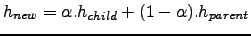 , where
  is going from 0
to 1 in "n-band" points from the parent/child boundaries). You should also select
the child minimum depth ("Hmin", it should be lower or equal to the parent minimum
depth), the maximum depth at the coast ("Hmax coast"), the number of selective
hanning filter passes for the deep regions ("n filter deep") and the number of
final hanning filter passes ("n filter final").
is going from 0
to 1 in "n-band" points from the parent/child boundaries). You should also select
the child minimum depth ("Hmin", it should be lower or equal to the parent minimum
depth), the maximum depth at the coast ("Hmax coast"), the number of selective
hanning filter passes for the deep regions ("n filter deep") and the number of
final hanning filter passes ("n filter final").
- "Interp forcing": It interpolates the parent surface forcing on the child grid.
Select the parent forcing file to be interpolated (e.g.
/Roms_tools/Run/ROMSFILES/roms_frc.nc). The child forcing file
roms_frc.nc.1 will be created. The parent surface fluxes are interpolated on the
child grid. You can use "Interp bulk" if you are using a bulk formula. In this
case, the parent bulk file (e.g. /Roms_tools/Run/ROMSFILES/roms_blk.nc)
will be interpolated on the child grid.
- "Interp initial": It interpolates parent initial conditions on the child grid.
Select the parent initial file (e.g.
/Roms_tools/Run/ROMSFILES/roms_ini.nc). The child initial file (e.g.
/Roms_tools/Run/ROMSFILES/roms_ini.nc.1) will be created. If the
topographies are different between the parent and the child grids, the child
initial conditions are vertically re-interpolated. In this case you should check if
the options "vertical corrections" and "extrapolations"
are selected. It is preferable to always use these options.
If there are parent biological fields in the initial files, they can be processed
automatically, we have to define the type of biological models: either NPZD-type
(NChlPZD, N2ChlPZD2 or N2P2Z2D2) then click on the 'Biol'
button, either PISCES biogeochemical model, then click on the
'Pisces' button. The fields needed for the initialization of
these biological model will be processed.
For information, in the case of NPZD type model, there are 4 more fields and in the
case of PISCES biogeochemical model, there is 8 more fields.
- "Interp dust": It interpolates parent Iron dust forcing file conditions on the
child grid. This is needed only in case of PISCES biogeochemical experiments.
Select the parent initial file (e.g.
/Roms_tools/Run/ROMSFILES/roms_frcbio.nc). The child initial file (e.g.
/Roms_tools/Run/ROMSFILES/roms_frcbio.nc.1) will be created.
- "Interp restart" generates a child restart file from
a parent restart file
(e.g. /Roms_tools/Run/ROMSFILES/roms_rst.nc). This can be done to "hot
start" a child model after the spin-up of the parent model. As in the case of
initial files generation, there is the possibility to compute ans write in the
nested restart file either the biological fields from NPZD-type biological model,
either the PISCES biogeochemical fields. For this purpose, click either on the
'Biol' button, either on the the 'Pisces'
button.
- You can click on "Create roms.in.*" to generate a child input file (roms.in.1)
from the parent input file and click on "Create AGRIF_FixedGrids.in" to generate a
AGRIF_FixedGrids.in file (the file which defines the child grid position in the
parent grid).
- "River" can be used to locate the river on the coast.
- "Interp clim" can be useful to generate boundary conditions to test the child
model alone. As in the case of restart an initial nested files generation, during
the eventual phase of creation of a nested clim file, the fields related to the
NPZD-type biological models or the PISCES one can be computed and written in the
nested clim file. As usual, click either on the 'Biol' button or
on the 'Pisces' button.
The ROMS nesting procedure needs a Fortran 95 compiler. For Linux PCs,
the Intel Fortran Compiler (ifort) is available at
http://www.intel.com/software/products/compilers/flin/noncom.htm. To be able to
compile ROMS with ifort, you should change the corresponding
comments in jobcomp.
To activate the AGRIF nesting procedure, define AGRIF in
/Roms_tools/Run/cppdefs.h. Moreover, to activate the AGRIF nesting with the
-way capability, define AGRIF and AGRIF_WAYS.
It is possible to edit the file AGRIF_FixedGrids.in. This file contains the child
grid positions (i.e. imin,imax,jmin,jmax) and coefficients of refinement. A first
line gives the number of children grids per parent (if AGRIF_STORE_BAROT_CHILD is
defined, only one child grid can be defined per parent grid). A second line gives the
relative position of each grid and the coefficient of refinement for each dimension.
Edit the input files roms.in.1, roms.in.2 , etc... to define correctly the file names
and the time steps. To run the model, simply type at the prompt: roms roms.in.
To visualize the ROMS model outputs for different grid levels,
change the value in the "child models" box
in roms_gui.
An operating coastal modeling system can be designed following the
assumption that large scale offshore dynamics are slow in comparison
to the coastal system. The lateral boundary conditions are interpolated
from the last available ECCO model outputs and are kept constant during
the ROMS simulation. ECCO model outputs are delayed by about two to four
weeks, but we suppose that they are still relevant for the present large
scale oceanic structure. The Global Forecast System (GFS) is used for the
surface forcing. A first day of simulation is run in hindcast mode. This
will provide the initial conditions for the next simulated day.
Using GFS as surface forcing and ECCO for the lateral boundary conditions,
a forecast of 7 days is conducted. A UNIX C-Shell script
( /Roms_tools/Run/run_roms_forecast.csh) manages
data downloading, the hindcast and forecast simulations
and datas storage.
The script run_roms_forecast.csh starts Matlab in
batch mode to download
with OPENDAP the lateral boundary conditions from ECCO and
the surface forcing from GFS. It interpolates the data on ROMS
grid and launches the hindcast and the forecast runs.
The script run_roms_forecast.csh should be edited to change the
directory pathways (HOME, RUNDIR, PATH, LD_LIBRAIRY_PATH, MATLAB,...).
The ROMS input files /Roms_tools/Run/roms_hindcast.in and
/Roms_tools/Run/roms_forecast.in should also be edited to change
the length of the time step and the number of time steps.
The ROMS input file roms_hindcast.in should be defined such as
the hindcast run duration
is 1 day and a restart file is generated at the end of the hindcast run.
The script run_roms_forecast.csh can be relaunched everyday in batch mode
using crontab.
ROMS solves the primitive equations in an Earth-centered rotating environment, based
on the Boussinesq approximation and hydrostatic vertical momentum balance. ROMS is
discretized in coastline- and terrain-following curvilinear coordinates. ROMS is a
split-explicit, free-surface ocean model, where short time steps are used to advance
the surface elevation and barotropic momentum, with a much larger time step used for
temperature, salinity, and baroclinic momentum. ROMS employs a special 2-way
time-averaging procedure for the barotropic mode, which satisfies the 3D continuity
equation (Shchepetkin and McWilliams, 2005). The specially designed predictor-corrector time step
algorithm used in ROMS allows a substantial increase in the permissible time-step
size.
ROMS has been designed to be optimized on shared memory parallel computer
architectures such as the SGI/CRAY Origin 2000. Parallelization is done by two
dimensional sub-domains partitioning. Multiple sub-domains can be assigned to each
processor in order to optimize the use of processor cache memory. This allow
super-linear scaling when performance growth even faster than the number of CPUs.
The third-order, upstream-biased advection scheme implemented in ROMS allows the
generation of steep gradients, enhancing the effective resolution of the solution for
a given grid size (Shchepetkin and McWilliams, 1998). Explicit lateral viscosity is null everywhere in the
model domain except in sponge layers near the open boundaries where it increases
smoothly close to the lateral open boundaries.
A non-local, K-profile planetary (KPP) boundary layer scheme (Large, 1994)
parameterizes the unresolved physical vertical subgrid-scale processes. If a lateral
boundary faces the open ocean, an active, implicit, upstream biased, radiation
condition connects the
model solution to the surroundings (Marchesiello et al., 2001).
More informations and model description can also be found in the SCRUM Manuel
(Hedström, K. S. , 1997) and a more recent User Manual on ROMS (Rutgers
version2.1), both written by Kate Hedström2.2 (Hedström, K. S. , 2009) 2.3. These documents are available on the
ROMS_AGRIF web site : http://roms.mpl.ird.fr in the documentation section.
To address the challenge of bridging the gap between near-shore and offshore
dynamics, a nesting capability has been added to ROMS and tested for the California
Upwelling System (Penven et al., 2006). The method chosen for embedded griding takes
advantage of the AGRIF (Adaptive Grid Refinement in Fortran) package
(Debreu and Blayo, 2008; Blayo and Debreu, 1999; Debreu and Vouland, 2003; Debreu and Blayo, 2003; Debreu, 2000). AGRIF is a Fortran 95 package for the
inclusion of adaptive mesh refinement features within a finite difference numerical
model. One of the major advantages of AGRIF in static-grid embedding is the ability
to manage an arbitrary number of fixed grids and an arbitrary number of embedding
levels.
Figure 2.1:
Temporal coupling between a parent and a child grid for a refinement factor
of 3. The coupling is done at the baroclinic time step.
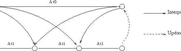 |
A recursive integration procedure manages the time evolution for the child grids
during the time step of the parent grids (Figure 2.1). In order
to preserve the CFL criterion, for a typical coefficient of refinement (say, a factor
of 3 for a 5 km resolution grid embedded in a 15 km grid), for each parent time step
the child must be advanced using a time step divided by the coefficient of refinement
as many time as necessary to reach the time of the parent (Figure
(2.1)). For simple 2-level embedding, the
procedure is as follows:
- Advance the parent grid by one parent time step.
- Interpolate the relevant parent variables in space and time to get the boundary
conditions for the child grid.
- Advance the child grid by as much child time steps as necessary
to reach the new parent model time.
- Update point by point the parent model by averaging the more accurate values of
the child model (in the case of 2-way embedding).
The recursive approach used in AGRIF allows the specification of any number of
embedding level. Other cpp keys are related to AGRIF, they are in
set_global_definitions.h and set_obc_definitions.h files. These ones are the
default conditions, are located in the ROMS_AGRIF code sources and should not be
edit by standard user.
2.2.2 AGRIF nesting procedure
To have a better undersatnding of the nesting capabilties of ROMS using AGRIF, it can
be useful to report to the homepage of the AGRIF project and papers related to its
application to ROMS.
- AGRIF homepage : http://www-ljk.imag.fr/MOISE/AGRIF/
- ROMS - AGRIF 1 way nesting : Evaluation and application of the ROMS 1-way,
embedding procedure to the central california upwelling system, (Penven et al., 2006)
- ROMS - AGRIF 2 way nesting: Two ways embedding algorithms for a split-explicit
free surface model. (Debreu et al , 2010)
2.3 Changelog since ROMS_AGRIF 1.1
- New diffusive-advection schemes : TS_SPLIT_UP3, Ref
(Marchesiello et al , 2009)
To avoid unacceptable spurious diapycnal mixing, a new advection scheme has been
proposed and validate : the RSUP3 scheme. The diffusion is split from advection and
is represented by a rotated biharmonic diffusion scheme with flow-dependent
hyperdiffusivity satisfying the Peclet constraint. The rotated diffusion operator
is designed for numerical stability, which includes improvements of linear
stability limits and a clipping method adapted to the sigma-coordinate.
This scheme induce a time step smaller than the third-order upstream biaised
diffusive advective scheme used in the version . It is activated by the use of
the cppkeys TS_SPLIT_UP3 cppdefs.h file.
To avoid numerical instabilities in the sponge where there is enhanced
diffusion/diffsuivity, a classical laplacian diffusion can be applied by the use of
the cppkey SPONGE_DIF2 and SPONGE_VIS2 in the cppdefs.h file.
- Two-way AGRIF nesting : AGRIF_2WAY, Ref. (Debreu et al , 2010)
As presented before, it is the capability of the fine grid to update data in the
coarse grid. With this procedure, we are now able to get the impact of high
resolution on the more coarser reolution, in a context of upscaling. To activate
the two ways nesting, you need to define the AGRIF and
AGRIF_2WAY cpp-keys.
- New bulk formulation : BULK_FAIRALL, Ref. (, )
A new bulk formulae has been set-up in the code, to compute surface wind stress and
surface net heat fluxes, as described in Fairall et al, 1996. (, ),
the use of this bulk formulae is activated by the cpp keys BULK_FAIRALL.
- Online diagnostics and I/O:
New diagnostics and outputs are now available in the ROMS_AGRIF  ., as
wind stresses, windspeed, and heat fluxes (latent, sensible, long-wave and solar
short wave). They can be written in the netCDF history and average files. Moreover,
bottom boundary layer thickness and euphotic depth layer in case of biological
experiments can be saved. For more information, you can refer at the section
2.6.
., as
wind stresses, windspeed, and heat fluxes (latent, sensible, long-wave and solar
short wave). They can be written in the netCDF history and average files. Moreover,
bottom boundary layer thickness and euphotic depth layer in case of biological
experiments can be saved. For more information, you can refer at the section
2.6.
Improvmement have also been carried out on the tracer and momentum equation term
diagnostics.
From now, the tracer equation terms are in dia.nc and dia_avg.nc
netcdf file with flags that permit to choose exactly the term
you want to write in the NetCDF files.
By default this diagnostics are written in a divergence flux form, (
 ,
,
 , ...) but they can be written in an "advective form"
:
, ...) but they can be written in an "advective form"
:
 ,
,
 , ... by using the DIAGNOSTICS_TS_ADV cpp key.
Some term have been added : the term integrated over the mixed layer depth (cppkeys
DIAGNOSTICS_TS_MLD. The mixed layer depth is computed online, from the
closure module.
, ... by using the DIAGNOSTICS_TS_ADV cpp key.
Some term have been added : the term integrated over the mixed layer depth (cppkeys
DIAGNOSTICS_TS_MLD. The mixed layer depth is computed online, from the
closure module.
The differents term of the tracer equation, that can be diagnose,
for each tracer, expressed in  , are:
- Time evolution term (called "rate" term)
- Zonal advective term
- Meridian advective term
- Vertical advective term
- Horizontal mixing term
- Vertical mixing term
- Nudging
 Surface forcing term (called Tforc term)
- In the case of use DIAGNOSTICS_TS_MLD some additional terms are
diagnosted :
- Time evolution term integrated over the surface mixed layer depth (MLD hereafter)
- Zonal advective term integrated over the MLD
- Meridian advective term integrated over the MLD
- Vertical advective term integrated over the MLD
- Horizontal mixing term integrated over the MLD
- Vertical mixing term integrated over the MLD
- Nudging Surface forcing term integrated over the MLD
- Entrainement term at the base of the mixed layer
Concerning the momentum equation term, the differents term of the equation can be
saved in history diaM.nc and average diaM_avg.nc netCDF files.
As the tracer, there are flags to choose exactly the term you want to write in the
netCDF file.
The differents terms of the momentum equation, expressed in  , that can be diagnose (for u and v)
are :
, that can be diagnose (for u and v)
are :
- Time evolution term (called "rate" term)
- Pressure gradient term
- Coriolis term
- Zonal advective
- Meridian advective
- Vertical advective
- Horizontal mixing
- Vertical mixing
2.4 Parameters description : param.h
In this section, we present the more important parameters to configure your own
run. These parameters are :
- Test case or realistic run:
...
#if defined BASIN  Test case
parameter (LLm0 , MMm0
 , N
, N )
)
#elif defined REGIONAL
Realistic run
# elif defined BENGUELA_LR
 parameter (LLm0
 , MMm0
 , N
, N )
)  BENGUELA_LR
# else
parameter (LLm0= , MMm0, N
 )
)
# endif
...
LLm0
MMm0
N
- Grid size:
- LLm0: Dimension (ghost points included) in the
 direction.
- MMm0: Dimension (ghost points included) in the
 direction.
- N: Number of
 -vertical points, in the vertical grid.
- Parallelization:
....
Domain subdivision parameters:
====== =========== ===========
NPP Maximum allowed number of parallel threads;
NSUB_X,NSUB_E Number of SHARED memory subdomains in XI- and
ETA-directions;
NNODES Total number of MPI processes (nodes);
NP_XI,NP_ETA Number of MPI subdomains in XI- and ETA-directions;
In the case of OpenMP parallelization, NPP is the number of cpu used in the
computation, in the case of MPI parallelization, it is equal to to NNODES.
AUTOTLING (implemented by Laurent Debreu): cppkeys that enable to compute the optimum
subdomains partition in terms of computation time.
- Tides:
...
#if defined SSH_TIDES || defined UV_TIDES
 integer Ntides
parameter (Ntides=8) Number of wave in
the total tidal signal
Number of wave in
the total tidal signal
#endif
...
2.5 CPP-keys description : cppdefs.h
In this section, we present the differents cpp keys used to define the numerical or
physical options in ROMS_AGRIF. These latters are ordered in differents sections and
described in Table 2.1.
Table 2.1:
Description of the CPP keys used in the cppdefs.h file
| TYPE |
CPP KEYS NAME |
| |
|
| TEST CASE |
|
| |
BASIN |
| |
CANYON_A |
| |
CANYON_B |
| |
GRAV_ADJ |
| |
INNERSHELF |
| |
OVERFLOW |
| |
SEAMOUNT |
| |
SHELFRONT |
| |
SOLITON |
| |
UPWELLING |
| |
INTERNAL |
| |
VORTEX |
| |
REGIONAL : realistric configuration |
Basic options |
| Configuration Name |
|
| |
BENGUELA |
| Parallelization |
|
| |
OPENMP |
| |
MPI |
| Embedding |
|
| |
AGRIF |
| |
AGRIF_2WAY |
| Open Boundary Conditions |
|
| |
TIDES |
| |
OBC_EAST |
| |
OBC_WEST |
| |
OBC_NORTH |
| |
OBC_SOUTH |
| Tides |
|
| |
TIDES |
| |
SSH_TIDES |
| |
UV_TIDES |
| |
TIDERAMP |
| Applications |
|
| |
BIOLOGY |
| |
FLOATS |
| |
STATIONS |
| |
PASSIVE_TRACER |
| |
SEDIMENT |
| |
BBL |
| |
|
More advanced options |
| Parallelization |
|
| |
PARALLEL_FILES |
| |
AUTOTILING |
| |
ETALON_CHECK |
| Model dynamics |
|
| |
SOLVE3D |
| |
UV_COR |
| |
UV_ADV |
| Grid configuration |
|
| |
CURVGRID |
| |
SPHERICAL |
| |
MASKING |
| Lateral Momentum Mixing |
|
| |
MIX_GP_UV |
| |
MIX_GP_UV |
| |
UV_VIS2 |
| |
UV_VIS4 |
| |
VIS_SMAGO |
| Lateral Tracer Mixing |
|
| |
MIX_GP_TS |
| |
MIX_S_TS |
| |
MIX_EN_TS |
| |
TS_DIF2 |
| |
TS_DIF4 |
| |
TS_SPLIT_UP3 |
| Nudging |
|
| |
ZNUDGING |
| |
M2NUDGING |
| |
M3NUDGING |
| |
TNUDGING |
| |
ROBUST_DIAG |
| Vertical Mixing |
|
| |
BODYFORCE |
| |
BVF_MIXING |
| |
LMD_MIXING |
| |
LMD_SKPP |
| |
LMD_BKPP |
| |
LMD_RIMIX |
| |
LMD_CONVEC |
| |
LMD_DDMIX |
| |
LMD_NONLOCAL |
| Equation of State |
|
| |
SALINITY |
| |
NONLIN_EOS |
| |
SPLIT_EOS |
| Surface Forcing |
|
| |
QCORRECTION |
| |
SFLX_CORR |
| |
DIURNAL_SRFLUX |
| |
BULK_FLUX |
| |
BULK_FAIRALL |
| |
BULK_LW |
| |
BULK_EP |
| |
BULK_SMFLUX |
| Sponge Layer |
|
| |
SPONGE |
| Lateral Forcing |
|
| |
|
| 1-Climatology strategy : 3D fields covering the whole domain |
|
|---|
| |
CLIMATOLOGY |
| |
ZCLIMATOLOGY |
| |
M2CLIMATOLOGY |
| |
M3CLIMATOLOGY |
| |
TCLIMATOLOGY |
| |
|
| 2-Boundary strategy : 1D fields only on OBC points |
|
|---|
| |
FRC_BRY |
| |
Z_FRC_BRY |
| |
M2_FRC_BRY |
| |
M3_FRC_BRY |
| |
T_FRC_BRY |
| Bottom Forcing |
|
| |
ANA_BSFLUX |
| |
ANA_BTFLUX |
| Point Sources - Rivers |
|
| |
PSOURCE |
| |
ANA_PSOURCE |
| Open Boundary Conditions |
|
| |
OBC_M2SPECIFIED |
| |
OBC_M2FLATHER |
| |
OBC_M2CHARACT |
| |
OBC_M2ORLANSKI |
| |
OBC_VOLCONS |
| |
OBC_M3ORLANSKI |
| |
OBC_M3SPECIFIED |
| |
OBC_TORLANSKI |
| |
OBC_TSPECIFIED |
| Input/Output and Diagnostics |
|
| |
AVERAGES |
| |
AVERAGES_K |
| |
DIAGNOSTICS_TS |
| |
DIAGNOSTICS_TS_ADV |
| |
DIAGNOSTICS_TS_MLD |
| |
DIAGNOSTICS_UV |
| BIOLOGY models |
|
| |
PISCES |
| |
BIO_NChlPZD |
| |
BIO_N2P2Z2D2 |
| |
BIO_N2ChlPZD2 |
|
|
Table 2.2:
Test Case related CPP keys
| CPP KEYS NAME |
Description |
| BASIN |
Must be defined for running the Basin Example. |
| CANYON_A |
Must be defined for running the Canyon_A Example. |
| CANYON_B |
Must be defined for running the Canyon_B Example. |
| GRAV_ADJ |
Must be defined for running the Gravitational Adjustment Example. |
| INNERSHELF |
Must be defined for running the Inner Shelf Example. |
| OVERFLOW |
Must be defined for running the Gravitational/Overflow Example. |
| SEAMOUNT |
Must be defined for running the Seamount Example. |
| SHELFRONT |
Must be defined for running the Shelf Front Example. |
| SOLITON |
Must be defined for running the Equatorial Rossby Wave Example. |
| UPWELLING |
Must be defined for running the Upwelling Example. |
| INTERNAL |
Must be defined for running the Internal tides example. |
| VORTEX |
Must be defined for running the Baroclinic Vortex Example. |
| REGIONAL |
Must be defined if running realistic regional simulations. |
|
|
Table 2.3:
Parallelization related CPP keys
| CPP KEYS NAME |
Description |
| OPENMP |
Activate the Open-MP parallelization protocol. |
| MPI |
Activate the MPI parallelization protocol. |
| PARALLEL_FILES |
Activate the I/O writing on multiprocessor. |
| AUTOTILING |
Activate the subdomains partitionning optimization. |
|
|
# ifdef MPI
#  undef PARALLEL_FILES
# endif
# undef AUTOTILING
Table 2.4:
Embedding related CPP keys
| CPP KEY NAME |
Description |
| AGRIF |
Activate the (1-WAYS) nesting capabilities. |
| AGRIF_2WAY |
Add the the 2-WAYS nesting (update of the parent grid solution by the child
grid solution) capabilities. |
|
|
Table 2.5:
Open Boundary Conditions (basic) related CPP keys
| CPP KEY NAME |
Description |
| OBC_EAST |
Open eastern boundary. |
| OBC_WEST |
Open western boundary. |
| OBC_SOUTH |
Open southern boundary. |
| OBC_NORTH |
Open northern boundary. |
|
|
Table 2.6:
Tides forcing related CPP keys
| CPP KEY NAME |
Description |
| TIDES |
Activate the forcing og tides at open-boundaries. |
| SSH_TIDES |
Define for processing sea surface elevation tidal data at the model boundaries. |
| UV_TIDES |
Define for processing ocean current tidal data at the model boundaries. |
| TIDERAMP |
Apply a ramping of the tidal current, (in general 2 days) at
initialization.
Warning! This should be off when restarting the model. |
|
|
# ifdef TIDES
# define SSH_TIDES
# define UV_TIDES
# define TIDERAMP
# endif
Table 2.7:
related CPP keys
| CPP KEY NAME |
Description |
| BIOLOGY |
Activate the biogeochemical module. |
| FLOATS |
Activate floats. |
| STATIONS |
Store model outputs for each time step at different station locations. |
| PASSIVE_TRACER |
Add a passive tracer. |
| SEDIMENT |
Activate the sediment module. |
| BBL |
Activate the bottom boundary layer module. |
|
|
# undef BIOLOGY
# undef FLOATS
# undef STATIONS
# undef PASSIVE_TRACER
# undef SEDIMENT
# undef BBL
Table 2.8:
Model dynamics related CPP keys
| CPP KEY NAME |
Description |
| SOLVE3D |
Define if solving 3D primitive equations. |
| UV_COR |
Activate Coriolis terms. |
| UV_ADV |
Activate advection terms. |
|
|
# define SOLVE3D
# define UV_COR
# define UV_ADV
# ifdef TIDES
# define SSH_TIDES
# define UV_TIDES
# define TIDERAMP
# endif
Table 2.9:
Model grid related CPP keys
| CPP KEY NAME |
Description |
| CURVGRID |
Activate curvilinear coordinate grid option. |
| SPHERICAL |
Activate longitude/latitude grid positioning. |
| MASKING |
Activate land masking in the domain. |
|
|
# define CURVGRID
# define SPHERICAL
# define MASKING
Table 2.10:
Lateral Momentum mixing related CPP keys
| CPP KEY NAME |
Description |
| MIX_GP_UV |
Activate mixing on geopotential (constant Z) surfaces. |
| MIX_S_UV |
Activate mixing on iso-sigma (constant sigma) surfaces. |
| UV_VIS2 |
Activate Laplacian horizontal mixing of momentum. |
| UV_VIS4 |
Activate Bilaplacian horizontal mixing of momentum. |
|
|
# define UV_VIS2
# define MIX_GP_UV
Table 2.11:
Lateral Tracer mixing related CPP keys
| CPP KEY NAME |
Description |
| MIX_GP_TS |
Activate mixing on geopotential (constant Z) surfaces. |
| MIX_S_TS |
Activate mixing on iso-sigma level surfaces. |
| MIX_EN_TS |
Activate mixing on isopygnal level surfaces. |
| TS_DIF2 |
Activate Laplacian horizontal mixing of tracer. |
| TS_DIF4 |
Activate Bilaplacian horizontal mixing of tracer. |
| TS_SPLIT_UP3 |
Activate the rotated split upstream advection-diffusion scheme for
tracer equation.
(Marchesiello et al , 2009) |
|
|
# define MIX_GP_TS
# define TS_DIF2
# undef TS_SPLIT_UP3
Table 2.12:
Nudging related CPP keys
| CPP KEY NAME |
Description |
| ZNUDGING |
Activate nudging layer for zeta. |
| M2NUDGING |
Activate nudging layer for barotropic velocities. |
| M3NUDGING |
Activate nudging layer for baroclinic velocities. |
| TNUDGING |
Activate nudging layer for tracer. |
| ROBUST_DIAG |
Activate strong tracer nudging in the interior for diagnostic simulations. |
|
|
The nudging layer has the same location than sponge layer. In the sponge/nudging
layer, the signal, tracers and momentum, is nudged towards climatology using a
nudging coefficient  expressed in
  , equal to the inverse of the
coefficient
, equal to the inverse of the
coefficient
 in the namelist roms.in
# define CLIMATOLOGY
# ifdef CLIMATOLOGY
.....
# define ZNUDGING
# define M2NUDGING
# define M3NUDGING
# define TNUDGING
# undef ROBUST_DIAG
# endif
Table 2.13:
Vertical mixing related CPP keys
| CPP KEY NAME |
Description |
| BODYFORCE |
Define if applying surface and bottom stresses as bodyforces |
| BVF_MIXING |
Activate a simple mixing scheme based on the Brunt-Väisälä frequency |
| LMD_MIXING |
Activate Large/McWilliams/Doney mixing (LMD-KPP closure) |
| LMD_SKPP |
Activate surface boundary layer KPP mixing (LMD-KPP closure) |
| LMD_BKPP |
Activate bottom boundary layer KPP mixing (LMD-KPP closure) |
| LMD_RIMIX |
Activate shear instability interior mixing (LMD-KPP closure) |
| LMD_CONVEC |
Activate convection interior mixing (LMD-KPP closure) |
| LMD_DDMIX |
Activate double diffusion interior mixing (LMD-KPP closure) |
| LMD_NONLOCAL |
Activate nonlocal transport (LMD-KPP closure) |
|
|
# undef BODYFORCE
# undef BVF_MIXING
# define LMD_MIXING
# ifdef LMD_MIXING
# define LMD_SKPP
# define LMD_BKPP
# define LMD_RIMIX
# define LMD_CONVEC
# undef LMD_DDMIX
# undef LMD_NONLOCAL
# endif
Table 2.14:
Equation of state related CPP keys
| CPP KEY NAME |
Description |
| SALINITY |
Define if using salinity. |
| NONLIN_EOS |
Activate the nonlinear equation of state. |
| SPLIT_EOS |
Activate the split of the nonlinear equation of state in a
adiabatic part and a compressible part for the reduction of pressure gradient errors
(Shchepetkin and McWilliams, 2003). |
|
|
# define SALINITY
# define NONLIN_EOS
# define SPLIT_EOS
Table 2.15:
Surface forcing related CPP keys
| CPP KEY NAME |
Description |
| BULK_FLUX |
Activate the bulk parametrization. |
| BULK_EP |
Activate the bulk parametrization for salinity fluxes. |
| BULK_LW |
Activate online long-wave radiation calculation using model SST. |
| BULK_SMFLUX |
Activate the bulk parametrization for surface momentum stress. |
| QCORRECTION |
Activate net heat flux correction. |
| SFLX_CORR |
Activate freshwater flux correction. |
| DIURNAL_SRFLUX |
Activate diurnal modulation of the short wave radiation flux. |
|
|
# define QCORRECTION
# define SFLX_CORR
# define DIURNAL_SRFLUX
# undef BULK_FLUX
# ifdef BULK_FLUX
# define LW_ONLINE
# define BULK_EP
# undef BULK_SMFLUX
# define DIURNAL_SRFLUX
# else
# define QCORRECTION
# define SFLX_CORR
# define DIURNAL_SRFLX
# endif
Table 2.16:
Sponge layer related CPP keys
| CPP KEY NAME |
Description |
| SPONGE |
Activate areas of enhanced viscosity/diffusion close to the
lateral open boundaries. |
|
|
Table 2.17:
Lateral forcing related CPP keys
| CPP KEY NAME |
Description |
| CLIMATOLOGY |
Activate processing of climatology data. |
| ZCLIMATOLOGY |
Activate processing of sea surface height climatology. |
| M2CLIMATOLOGY |
Activate processing of barotropic velocities climatology. |
| M3CLIMATOLOGY |
Activate processing of baroclinic velocities climatology. |
| TCLIMATOLOGY |
Activate processing of tracer climatology. |
| FRC_BRY |
Activate direct boundary forcing |
| Z_FRC_BRY |
Activate boundary forcing for zeta. |
| M2_FRC_BRY |
Activate boundary forcing for barotropic velocities. |
| M3_FRC_BRY |
Activate boundary forcing for baroclinic velocities |
| T_FRC_BRY |
Activate boundary forcing for tracers. |
|
|
# define CLIMATOLOGY
# ifdef CLIMATOLOGY
# define ZCLIMATOLOGY
# define M2CLIMATOLOGY
# define M3CLIMATOLOGY
# define TCLIMATOLOGY
# ...
# endif
# undef FRC_BRY
# ifdef FRC_BRY
# define Z_FRC_BRY
# define M2_FRC_BRY
# define M3_FRC_BRY
# define T_FRC_BRY
# endif
Table 2.18:
Bottom forcing related CPP keys
| CPP KEY NAME |
Description |
| ANA_BSFLUX |
Define if using analytical bottom salinity flux |
| ANA_BTFLUX |
Define if using analytical bottom temperature flux. |
|
|
# define ANA_BSFLUX
# define ANA_BTFLUX
Table 2.19:
Point Sources and Rivers related CPP keys
| CPP KEY NAME |
Description |
| PSOURCES |
Define if using point sources (rivers) |
| ANA_PSOURCES |
Define if using analytical vertical profiles for the point sources
(using fluxes defined in roms.in) |
|
|
# undef PSOURCE
# undef ANA_PSOURCE
Table 2.20:
Open Boundary Condition related CPP keys
| CPP KEY NAME |
Description |
| OBC_VOLCONS |
Activate mass conservation enforcement at open boundaries. |
| OBC_M2SPECIFIED |
Activate specified open boundary conditions for ubar and vbar. |
| OBC_M2ORLANSKI |
Activate 2D radiation open boundary conditions for ubar and vbar. |
| OBC_M2FLATHER |
Activate Flather open boundary conditions for ubar and vbar. |
| OBC_M2CHARACT |
Activate open boundary conditions based on characteristic methods. |
| OBC_M3SPECIFIED |
Activate specified open boundary conditions for u and v. |
| OBC_M3ORLANSKI |
Activate 2D radiation open boundary conditions for u and v. |
| OBC_M3CHARACT |
Activate open boundary conditions based on characteristic methods
for u and v. |
| OBC_TSPECIFIED |
Activate specified open boundary conditions for tracers. |
| OBC_TORLANSKI |
Activate 2D radiation open boundary conditions for tracers. |
| OBC_TUPWIND |
Activate upwind open boundary conditions for tracers. |
|
|
# ifdef TIDES
# define OBC_M2FLATHER
# else
# undef OBC_M2SPECIFIED
# undef OBC_M2FLATHER
# define OBC_M2CHARACT
# undef OBC_M2ORLANSKI
# ifdef OBC_M2ORLANSKI
# define OBC_VOLCONS
# endif
# endif
# define OBC_M3ORLANSKI
# define OBC_TORLANSKI
# undef OBC_M3SPECIFIED
# undef OBC_TSPECIFIED
Table 2.21:
I/O related CPP keys
| CPP KEY NAME |
Description |
| AVERAGES |
Define if writing out time-averaged data. |
| AVERAGES_K |
Define if writing out time-averaged vertical mixing. |
| DIAGNOSTICS_TS |
Define if writing out tendency terms for the tracer equations. |
| DIAGNOSTICS_TS_ADV |
Activate advection formulation for tendency term for the
tracer equations. |
| DIAGNOSTICS_TS_MLD |
Activate integration over the mixed-layer (MLD) for the
tendency term for the tracer equation. |
| DIAGNOSTICS_UV |
Define if writing out tendency terms for the momentum equations. |
|
|
# define AVERAGES
# define AVERAGES_K
# undef DIAGNOSTICS_TS
# undef DIAGNOSTICS_UV
# ifdef DIAGNOSTICS_TS
# undef DIAGNOSTICS_TS_ADV
# undef DIAGNOSTICS_TS_MLD
# endif
Table 2.22:
Biology model related CPP keys
| CPP KEY NAME |
Description |
| PISCES |
Activate PISCES biogeochemical model |
| BIO_NChlPZD |
Activate idealized 4 compartiments NPZD type model |
| BIO_N2PZD2 |
Activate idealized 6 compartiments NPZD type model |
| BIO_N2ChlP2Z2D2 |
Activate idealized 8 compartiments NPZD type model |
|
|
# ifdef BIOLOGY
# undef PISCES
# define BIO_NChlPZD
# undef BIO_N2P2Z2D2
# undef BIO_N2ChlPZD2
# endif
2.6 Namelist description : roms.in
title:
South Benguela TEST MODEL
time_stepping: NTIMES dt[sec] NDTFAST NINFO


S-coord: THETA_S, THETA_B, Hc (m)


grid: filename
roms_grd.nc
forcing: filename
roms_frc.nc
bulk_forcing: filename
roms_bulk.nc
climatology: filename
roms_clm.nc
boundary: filename
roms_bry.nc
initial: NRREC filename
roms_ini.nc
restart: NRST, NRPFRST / filename

roms_rst.nc
history: LDEFHIS, NWRT, NRPFHIS / filename


roms_his.nc
averages: NTSAVG, NAVG, NRPFAVG / filename
roms_avg.nc
primary_history_fields: zeta UBAR VBAR U V wrtT(1:NT)
T T T T T  *T
*T
auxiliary_history_fields: rho Omega W Akv Akt Aks HBL HBBL Bostr Wstr Ustr Vstr rsw rlw lat sen HEL
F F T F T F T T T T T T  *F
*F
primary_averages: zeta UBAR VBAR U V wrtT(1:NT)
T T T T T *T
auxiliary_averages: rho Omega W Akv Akt Aks HBL HBBL Bostr Wstr Ustr Vst rsw rlw lat sen HEL
F T T F T F T T T T T T *F
rho0:

lateral_visc: VISC2, VISC4 [ /sec for all]

tracer_diff2: TNU2(1:NT) [ /sec for all]

tracer_diff4: TNU4(1:NT) [ /sec for all]

vertical_mixing: Akv_bak, Akt_bak [/sec]
d  d
d
bottom_drag: RDRG [m/s], RDRG2, Zob [m], Cdb_min, Cdb_max
 d
d d
d .d .d
.d .d .d
.d
gamma2:
 d
d
sponge: X_SPONGE [m], V_SPONGE [ / sec]


nudg_cof: TauT_in, TauT_out, TauM_in, TauM_out [days for all]


diagnostics: ldefdia nwrtdia nrpfdia /filename
T
roms_dia.nc
diag_avg: ldefdia_avg ntsdia_avg nwrtdia_avg nprfdia_avg /filename
T 0
roms_dia_avg.nc
diag D_history_fields: diag_tracersD(1:NT)
*T
diagD_history_fields: diag_tracersD(1:NT)
*T
diagD_average_fields: diag_tracersD_avg(1:NT)
*T
diagD_average_fields: diag_tracersD_avg(1:NT)
*T
diagnosticsM: ldefdiaM nwrtdiaM nrpfdiaM /filename
T
roms_diaM.nc
diagM_avg: ldefdiaM_avg ntsdiaM_avg nwrtdiaM_avg nprfdiaM_avg /filename
T
roms_diaM_avg.nc
diagM_history_fields: diagM_momentum(1:2)
T T
diagM_average_fields: diagM_momentum_avg(1:2)
T T
diagnostics_bio: ldefdiabio nwrtdiabio nrpfdiabio /filename
T
roms_diabio.nc
diagbio_avg: ldefdiabio_avg ntsdiabio_avg nwrtdiabio_avg nprfdiabio_avg
/filename
T
roms_diabio_avg.nc
biology: forcing file
roms_frcbio.nc
sediments: input file
sediment.in
sediment_history_fields: bed_thick bed_poros be3d_fra(sand,silt)
T F T T
bbl_history_fields: Abed Hripple Lripple Zbnot Zbapp Bostrw
T F F T F T
floats: LDEFFLT, NFLT, NRPFFLT / inpname, hisname
T 
floats.in
floats.nc
float_fields: Grdvar Temp Salt Rho Vel
F F F F F
stations: LDEFSTA, NSTA, NRPFSTA / inpname, hisname
T 
stations.in
stations.nc
station_fields: Grdvar Temp Salt Rho Vel
T T T T T
psource: Nsrc Isrc Jsrc Dsrc Qbar [m3/s] Lsrc Tsrc

 T T
T T 
 0 T T
0 T T
Table 2.23:
Description of the roms.in file
| KEYWORDS |
DESCRIPTIONS |
| title |
|
|---|
| |
|
| time_stepping |
|
|---|
| |
NTIMES : Number of time step for the run. |
| |
dt : Baroclinic time step for the run [in s] |
| |
NDTFAST : Number of bariotropic time step in one baroclinic time step. |
| |
NINFO : frequency of output in time steps. |
| S-coord |
|
|---|
| |
THETA_S:  -coordinate surface control parameter, -coordinate surface control parameter,
 theta_s theta_s  |
| |
THETA_B: -coordinate bottom control parameter,
theta_b |
| |
Hc(m): Width of the surface or bottom topography layer in which higher vertical
resolution is required during stretching. |
| grid |
|
|---|
| |
/filename: Name of the grid file. |
| |
|
| forcing |
|
|---|
| |
/filename: Name of the surface forcing file : wind stress, atmospheric fluxes (E-P,
net heat fluxes) and nudging coefficients towards dQ/dSST. |
| |
|
| bulk_forcing |
|
|---|
| |
/filename: Name of the bulk forcing file for atmospheric forcings. |
| climatology |
|
|---|
| |
/filename: Name of the open boundaries conditions (t, s,  , ,  , ,  , ,
 ). These files are 3d in space, covering the whole domain. ). These files are 3d in space, covering the whole domain. |
| |
|
| boundary |
|
|---|
| |
/filename: Name of the open boundaries conditions (T, S, , , ,
). These files are covering only the open-boundaries slices, inducing files much
smaller than the ``climatology'' ones. |
| |
|
| initial |
|
|---|
| |
NRREC: Record number of the restartfile to read as the initial conditions. |
| |
/filename: Name of the file containing initial state. |
| |
|
| restart |
|
|---|
| |
NRST: Frequency of writing |
| |
NRPFRST 0: writing several records every NRST time steps. -1: overwriting record
every NRST time steps |
| |
/filename |
| |
|
| history |
|
|---|
| |
LDEFHIS: flag (T/F) if writing history files |
| |
NWRT: Frequency of writing |
| |
NRPFHIS: 0: writing several records every NWRT time steps. -1: overwriting record
every NRST time steps |
| |
/filename: Name of the gistory file |
| |
|
| averages |
|
|---|
| |
NTSAVG: Starting timestep for the accumulation of output time-averaged data. For
instance, you might want to average over the last day of a thirty-day run. |
| |
NAVG: frequency of writing |
| |
NRPFAVG: 0: writing several records every NWRT time steps. -1: overwriting record
every NAVG time steps |
| |
/filename |
| |
|
| primary_history _fields |
|
|---|
| |
Flags of written primary variables in history NetCDF file |
| |
|
| auxiliary_history _fields |
|
|---|
| |
Flags of written auxiliary variables in history NetCDF file |
| |
|
| primary_averages |
|
|---|
| |
Flags of written primary variables in history NetCDF file |
| |
|
| auxiliary_averages |
|
|---|
| |
Flags of written variables in average NetCDF file |
| |
|
| rho0 |
Mean density used in the Boussinesq equation. |
|---|
| |
|
| lateral_visc |
|
|---|
| |
VISC2: Laplaplacian background viscosity |
| |
VISC4: Bilaplacian background viscosity |
| |
|
| tracer_diff2 |
|
|---|
| |
TNU2(1:NT): Laplacian background diffusivity for each tracer. |
| |
|
| tracer_diff4 |
|
|---|
| |
TNU4(1:NT): Laplacian background diffusivity for each tracer. |
| |
|
| vertical_mixing |
|
|---|
| |
Coefficient in case of use of analytical vertical mixing scheme. |
| |
|
| bottom_drag |
|
|---|
| |
RDRG [m/s]: Drag coefficient in case of linear bottom stress formulation. |
| |
|
| |
RDRG2: Drag coefficient in case of constant quadratic bottom stress formulation. |
| |
|
| |
Zob [m]: Rugosity length in case of Von-Karman quadratic bottom stress formulation |
| |
Cdb_min: Minimum value of the drag coefficient in case Von-Karman quadratic bottom stress formulation. |
| |
Cdb_max: Maximum value of the drag coefficient in case Von-Karman quadratic bottom stress formulation. |
| |
|
| gamma2 |
|
|---|
| |
Free slip boundary condition. 1 mean free slip condition are ON. |
| |
|
| sponge |
|
|---|
| |
X_SPONGE [m]: widthness of the sponge layers. |
| |
V_SPONGE [ ]: Value of the viscosity and diffusity enhanced value at
the boundary point in the nudging/sponge layer. These value are enhanced following a
linear profil in the sponge/nudging layer, from the interior value to the max value
V_SPONGE at boundary. ]: Value of the viscosity and diffusity enhanced value at
the boundary point in the nudging/sponge layer. These value are enhanced following a
linear profil in the sponge/nudging layer, from the interior value to the max value
V_SPONGE at boundary. |
| |
|
| nudg_cof |
|
|---|
| |
TauT_in [days]: Nudging time scale for tracer signal going inward the
domain. This coefficient is used at boundary point and impose a
strong nudging towards climatology external data. |
| |
|
| |
TauT_out [days]: Nudging time scale for tracer signal going outward the domain. This coefficient is used at boundary point and impose a
smooth nudging towards climatology external data. This coefficient is also used in
the nudging/sponge layer to add a smooth nudging towards data. This is on only if the
CLIMATOLOGY boundary stategy is used, not the BRY one. |
| |
|
| |
TauM_in [days]: Same as above, but concerning the momentum equations. |
| |
|
| |
TauM_out [days]: Same as above, but concerning the momentum equations. |
| |
|
| diagnostics |
|
|---|
| |
ldefdia: Boolean flag to activate the tracer equation "snap-shot" diagnostic file writing |
| |
nwrtdia: Frequency of writing |
| |
nrpfdia: nrpfdia: 0: writing several records every nwrtdia time steps. -1: overwriting record
every nwrtdia time steps |
| |
/filename: Name of the file tracer equation diagnostic file. |
| diag_avg |
|
|---|
| |
ldefdia_avg: Boolean flag to activate the tracer equation average diagnostic file writing |
| |
ntsdia_avg: Starting timestep for the accumulation of output time-averaged data. For
instance, you might want to average over the last day of a thirty-day run. |
| |
nwrtdia_avg: Frequency of writing and average time. |
| |
nprfdia_avg: nrpfdia_avg: 0: writing several records every nwrtdia_avg time steps. -1: overwriting record
every nwrtdia_avg time steps |
| |
/filename: Name of the file tracer equation average diagnostic file. |
| |
|
| diag3D_history _fields |
|
|---|
| |
Boolean flag to choose which tracer equation (temp, salt, etc ...) is computed in
diagnostics and saved in NetCDF file. Terms are 3D |
| |
|
| diag2D_history _fields |
|
|---|
| |
Boolean flags to choose which tracer equation, after mixed layer depth integration (cf
DIAGNOSTICS_TS_MLD) is computed in diagnostics and saved in NetCDF file. Terms are 2D |
| |
|
| diag3D_average _fields |
|
|---|
| |
Boolean flag to choose which tracer equation (temp, salt, etc ...) is computed in
diagnostics and saved in NetCDF file. Terms are 3D and are averaged over the diagnostic TS
period defined as above, as nwrtdia |
| |
|
| diag2D_average _fields |
|
|---|
| |
Boolean flags to choose which tracer equation, after mixed layer depth integration (cf
DIAGNOSTICS_TS_MLD) is computed in diagnostics and saved in NetCDF file. Terms are 2D
and are averaged over the diagnostic period defined as above, as nwrtdia |
| |
|
| diagnosticsM |
Same format as diagnostics but for the momentum equation. |
|---|
| |
ldefdiaM: |
| |
nwrtdiaM: |
| |
nrpfdiaM: |
| |
/filename: |
| |
|
| diagM_avg |
Same format as diag_avg but for the momentum equation. |
|---|
| |
ldefdiaM_avg: |
| |
ntsdiaM_avg: |
| |
nwrtdiaM_avg: |
| |
nprfdiaM_avg: |
| |
/filename |
| |
|
| diagM_history _fields |
|
|---|
| |
Boolean flag to choose which momentum equations are diagnosed and saved in NetCDF
file. The diagnostics terms are 3D. |
| |
|
| diagM_average _fields |
|
|---|
| |
Boolean flag to choose which momentum equation are diagnosed and saved in NetCDF
file. The diagnostics terms are 3D and are averaged over the diagnostic
period defined above, as nwrtdiaM_avg. |
| |
|
| diagnosticsM_bio |
Same format as diagnostics |
|---|
| |
ldefdiabio |
| |
nwrtdiabio |
| |
nrpfdiabio |
| |
/ filename |
| |
|
| diagbio_avg |
Same format as diag_avg |
|---|
| |
ldefdiabio_avg |
| |
ntsdiabio_avg |
| |
nwrtdiabio_avg |
| |
nprfdiabio_avg |
| |
/ filename |
| |
|
| biology |
|
|---|
| |
Name of the file containing the Iron dust forcing if using PISCES biogeochemical
mode. |
| |
|
| sediments |
|
|---|
| |
|
| sediment_history _fields |
|
|---|
| |
bed_thick |
| |
bed_poros |
| |
bed_fra(sand,silt) |
| |
|
| bbl_history_fields |
|
|---|
| |
Abed |
| |
Hripple |
| |
Lripple |
| |
Zbnot |
| |
Zbapp |
| |
Bostrw |
| |
|
| floats |
Lagrangian floats application |
|---|
| |
Same format as diagnostics |
| |
LDEFFLT |
| |
NFLT |
| |
NRPFFLT |
| |
/ inpname, hisname |
| |
|
| floats_fields |
|
|---|
| |
Type of fields computed for each lagrangian floats. |
| |
|
| station_fields |
Fixed station application. |
|---|
| |
Same format as diagnostics |
| |
LDEFSTA |
| |
NSTA |
| |
NRPFSTA |
| |
/ inpname, hisname |
| |
|
| psource |
|
|---|
| |
Nsrc |
| |
Isrc |
| |
Jsrc |
| |
Dsrc |
| |
Qbar [m3/s] |
| |
Lsrc |
| |
Tsrc |
| |
|
|
|
-
Aumont, O.
2005.
PISCES biogeochemical model description.
Internal report, 36 pages
-
-
Beckmann, A., Haidvogel, D.B.,
1993.
Numerical simulation of flow around a tall
isolated seamount. Part I: Problem formulation
and model accuracy.
Journal of Physical Oceanography
23,
1736-1753.
-
-
Blanke, B., Roy, C., Penven, P., Speich, S.,
McWilliams, J.C., Nelson, G.,
2002.
Linking wind and upwelling interannual variability in a
regional model of the southern Benguela,
Geophysical Research Letters
29,
2188-2191.
-
-
Blayo, E., Debreu, L.,
1999.
Adaptive mesh refinement for finite-difference
ocean models: First experiments.
Journal of Physical Oceanography
29, 1239-1250.
-
-
Carton, J.A., Giese, B.S., Grodsky, S.A., 2005.
Sea level rise and the warming of the oceans in the
Simple Ocean Data Assimilation (SODA) ocean reanalysis.
Journal of Geophysical Research
110, C09006, doi:10.1029/2004JC002817.
-
-
Casey, K.S., Cornillon, P., 1999.
A comparison of satellite and in situ based
sea surface temperature climatologies.
Journal of Climate
12, 1848-1863.
-
-
Conkright, M.E., R.A. Locarnini, H.E. Garcia, T.D. O Brien,
T.P. Boyer, C. Stephens, J.I. Antonov, 2002.
World Ocean Atlas 2001: Objective Analyses, Data Statistics,
and Figures, CD-ROM Documentation.
National Oceanographic Data Center,
Silver Spring, MD,
17 pp.
-
-
Da Silva, A.M., Young, C.C., Levitus, S.
1994.
Atlas of surface marine data 1994,
Vol. 1,
algorithms and procedures,
NOAA Atlas NESDIS 6,
U. S. Department of Commerce,
NOAA,
NESDIS,
USA,
74 pp.
-
-
Debreu, L.,
2000.
Raffinement adaptatif de maillage et méthodes de zoom -
application aux modèles d'océan,
2000,
Ph.D. thesis,
Université Joseph Fourier,
Grenoble.
-
-
Debreu, L., Blayo, E.,
2003.
AGRIF: Adaptive Grid Refinement In Fortran.
submitted to ACM Transactions on Mathematical Software - TOMS.
-
-
Debreu, L., Vouland, C.,
2003.
AGRIF: Adaptive Grid Refinement In Fortran.
[Available online http://www-lmc.imag.fr/IDOPT/AGRIF/index.html].
-
-
Debreu, L., Blayo, E.,
2008.
Special Issue on Multi-Scale Modelling:
Nested Grid and Unstructured Mesh Approaches.
Ocean Dynamics
58, 415-428.
doi 10.1007/s10236-008-0150-9
-
-
Debreu, L., Marchesiello, P., Penven, P.
2010.
Two ways embedding algorithms for a split-explicit free surface model.
Ocean Modelling,
submitted
-
-
Di Lorenzo, E., Miller, A.J., Neilson, D.J.,
Cornuelle, B.D., Moisan, J.R.,
2003.
Modeling observed California Current mesoscale eddies and
the ecosystem response .
International Journal of Remote Sensing,
in press.
-
-
Egbert, G., Erofeeva, S., 2002.
Efficient inverse modeling of barotropic ocean tides,
Journal of Atmospheric and Oceanic Technology
19,
183-204.
-
-
Fairall, C.W., E.F. Bradley, E.F., Rogers D.P., Edson J.B., Young
G.S.
1996.
Bulk parameterization of air-sea fluxes for topical ocean-global
atmosphere Coupled-Ocean Atmosphere Response Experiment,
JGR,
101,
3747-3764
-
-
Flather, R.A., 1976.
A tidal model of the northwest European continental shelf.
Mémoires de la Société Royale des Sciences de Liège,
10,
141-164.
-
-
Haidvogel, D.B., Arango, H.G., Hedstrom, K. , Beckmann, A.,
Malanotte-Rizzoli, P., Shchepetkin, A.F.,
2000.
Model Evaluation Experiments in the North Atlantic Basin:
Simulations in Nonlinear Terrain-Following Coordinates.
Dynamics of Atmospheres and Oceans
32 ,
239-281.
-
-
Haney, R.L.,
1991.
On the pressure force over steep
topography in sigma coordinate ocean models.
Journal of Physical Oceanography
21,
610-619.
-
-
Hedstrom, K. S., 1997.
SCRUM Manuel,
Institute of Marine and Coastal Sciences, Rutgers University, USA
-
-
Hedstroem, K. S., 2009.
DRAFT Technical Manual for a Coupled Sea-Ice/Ocean Circulation Model
(Version 3),
U.S Department of the Interior, Mineral Management Service, Anchorage,
Alaska,
Arctic Region Supercomputing Center, University of Alaska Fairbanks,
Contract M07PC13368
-
-
Jackett, D.R., McDougall, T.J.,
1995.
Minimal Adjustment of Hydrostatic Profiles to
Achieve Static Stability.
Journal of Atmospheric and Oceanic Technology
12,
381-389.
-
-
Large, W.G., McWilliams, J.C., Doney, S.C.,
1994.
Oceanic vertical mixing: a review and a model
with a nonlocal boundary layer parameterization.
Reviews in Geophysics
32,
363-403.
-
-
MacCready, P. M., R. D. Hetland, W. R. Geyer,
Long-Term Isohaline Salt Balance in an Estuary.
Continental Shelf Research, 22, 1591-1601.
-
-
Marchesiello, P., Debreu, L., Couvelard, X.
2009.
Spurious diapycnal mixing in terrain-following coordinate models: The problem
and a solution.
Ocean Modelling
26,
156-169.
-
-
Marchesiello, P., McWilliams, J.C., Shchepetkin, A.,
2001.
Open boundary condition for long-term integration of regional oceanic
models.
Ocean Modelling
3,
1-21.
-
-
Marchesiello, P., McWilliams, J.C., Shchepetkin, A.,
2003.
Equilibrium structure and dynamics of the California Current System.
Journal of Physical Oceanography
33,
753-783.
-
-
Penven, P., Roy C., Lutjeharms, J.R.E.,
Colin de verdière, A., Johnson, A., Shillington, F.,
Fréon, P., Brundrit, G.,
2001.
A regional hydrodynamic model of the Southern Benguela.
South African Journal of Science
97,
472-476.
-
-
Penven, P., Debreu, L., Marchesiello, P., McWilliams, J.C.,
2006.
Application of the ROMS embedding procedure for the Central
California Upwelling System.
Ocean Modelling
12, 157-187.
-
-
Penven, P., Marchesiello, P., Debreu, L., Lefèvre, J.,
2007.
Software tools for pre- and post-processing of oceanic regional
simulations.
Environmental Modelling and Software,
in press.
-
-
Reynolds, R.W., Smith, T.M., 1994.
Improved global sea surface temperature
analyses using optimum interpolation.
Journal of Climate.
7, 929-948.
-
-
Shchepetkin, A.F., McWilliams, J.C.,
1998.
Quasi-monotone advection schemes based on explicit locally
adaptive dissipation.
Monthly Weather Review
126,
1541-1580.
-
-
Shchepetkin, A.F., McWilliams, J.C.,
2003.
A method for computing horizontal pressure-gradient force
in an ocean model with a non-aligned vertical coordinate.
Journal of Geophysical Research
108.
-
-
Shchepetkin, A.F., McWilliams, J.C.,
2005.
Regional Ocean Model System: a split-explicit ocean model with a
free-surface and topography-following vertical coordinate.
Ocean Modelling
9, 347-404.
-
-
Smith, W.H.F., Sandwell, D.T.,
1997.
Global seafloor topography from satellite altimetry and ship depth soundings.
Science
277,
1957-1962.
-
-
Stammer, D., Davis, R., Fu, L.L., Fukumori, I., Giering, R., Lee, T.,
Marotzke, J., Marshall, J., Menemenlis, D., Niiler, P., Wunsch, C.,
Zlotnicki., V., 1999.
The consortium for estimating the circulation and
climate of the ocean (ECCO) - Science goals and task plan - Report
N
 1.
Techical report,
Jet Propulsion Laboratory - Massachusetts Institute of
Technology - Scripps Institution of Oceanography.
1.
Techical report,
Jet Propulsion Laboratory - Massachusetts Institute of
Technology - Scripps Institution of Oceanography.
-
This document was generated using the
LaTeX2HTML translator Version 2002-2-1 (1.71)
Copyright © 1993, 1994, 1995, 1996,
Nikos Drakos,
Computer Based Learning Unit, University of Leeds.
Copyright © 1997, 1998, 1999,
Ross Moore,
Mathematics Department, Macquarie University, Sydney.
The command line arguments were:
latex2html -split 0 -white -show_section_numbers -no_navigation doc.tex
The translation was initiated by Gildas Cambon on 2010-07-20
Footnotes
- ... experiments1.1
- These routines use add_dic.m, add_doc.m, add_fer.m, add_o2.m, add_talk.m, add_sio3.m,
add_ini_dic.m, add_ini_doc.m, add_ini_fer.m, add_ini_o2.m, add_ini_talk.m, add_ini_po4.m, add_ini_sio3.m
- ...
version2.1
- http://myroms.org
- ... Hedström2.2
- Kate
Hedström, University of Alaska Fairbanks, Center for Arctic Region Supercomputing
Center, University of Alaska Fairbanks,
- ...hedstroem2009 2.3
- Many
thanks to Kate Hedstroëm for this work.
Gildas Cambon
2010-07-20
![\includegraphics[width=1\textwidth]{Figures/dustdepo_surface.eps}](img45.png)
![\includegraphics[width=12cm]{Figures/nestgui_entrance.eps}](img57.png)
![\includegraphics[width=1\textwidth]{Figures/nestgui_vizu.eps}](img58.png)